
International Journal of Computational Intelligence Systems

Volume 13, Issue 1, 2020, Pages 822 - 851

Group Decision-Making Using Complex q-Rung Orthopair Fuzzy Bonferroni Mean

Authors
Peide Liu1, *, ORCID, Zeeshan Ali2, Tahir Mahmood2, ORCID, Nasruddin Hassan3, ORCID
1School of Management Science and Engineering, Shandong University of Finance and Economics, Jinan 250015, China
2Department of Mathematics and Statistics, International Islamic University, Islamabad 44000, Pakistan
3School of Mathematical Sciences, Faculty of Science and Technology, Universiti Kebangsaan Malaysia, Bangi 43600, Malaysia
*Corresponding author. Email: peide.liu@gmail.com
Corresponding Author
Peide Liu
Received 3 April 2020, Accepted 12 May 2020, Available Online 22 June 2020.
DOI
10.2991/ijcis.d.200514.001How to use a DOI?
Keywords
Complex q-rung orthopair fuzzy sets; Bonferroni mean operators; Multi-attribute group decision-making problems
Abstract

Complex q-rung orthopair fuzzy set (CQROFS), as a modified notion of complex fuzzy set (CFS), is an important tool to cope with awkward and complicated information. CQROFS contains two functions which are called truth grade and falsity grade by the form of complex numbers belonging to unit disc in a complex plane. The condition of CQROFS is that the sum of q-powers of the real part (Also for imaginary part) of the truth grade and real part (Also for imaginary part) of the falsity grade is limited to the unit interval. Bonferroni mean (BM) operator is an important and meaningful concept to examine the interrelationships between the different attributes. Keeping the advantages of the CQROFS and BM operator, in this manuscript, the complex q-rung orthopair fuzzy BM (CQROFBM) operator, complex q-rung orthopair fuzzy weighted BM (CQROFWBM) operator, complex q-rung orthopair fuzzy geometric BM (CQROFGBM) operator, and complex q-rung orthopair fuzzy weighted geometric BM (CQROFWGBM) operator are proposed, and some properties are discussed, further, based on the CQROFWGBM operator, a multi-attribute group decision-making (MAGDM) method is developed, and the ranking results are examined by score function. Finally, we give some numerical examples to verify the rationality of the established method, and show its advantages by comparative analysis with some existing methods.

Copyright
© 2020 The Authors. Published by Atlantis Press SARL.
Open Access
This is an open access article distributed under the CC BY-NC 4.0 license (http://creativecommons.org/licenses/by-nc/4.0/).

1. INTRODUCTION

Intuitionistic fuzzy set (IFS) was explored by Atanssove [1] as a modified notion of the fuzzy set (FS) [2], and it contains two functions called as truth grade and falsity grade, whose sum is not exceeded to the unit interval. IFS is an effective tool to describe the complicated fuzzy information, and it has received extensive attention. For example, Garg and Kumar [3] explored a novel exponential distance and TOPSIS methods for interval-valued IFS; Garg and Kaur [4] investigated the extended TOPSIS method using cubic IFS and applied it to multi-attribute group decision-making (MAGDM) problem; Joshi [5] examined a new decision-making method based on IFS and applied it to fault detection in a machine; Kumar [6] explored intuitionistic fuzzy zero point method for solving type-2 intuitionistic fuzzy transportation problem; Alcantud et al. [7] aggregated the finite chains of IFSs to deal with temporal IFSs; Kumar [8] evaluated the models for examining the optimization problems using IFSs. Yue [9] applied a projection-based approach based on IFSs to software quality evaluation.

However, the scope of the IFS is narrow because it should satisfy the condition that the sum of truth and falsity grades is bounded to the unit interval. If some decision makers (DMs) provide such kind of information whose sum is not limited to the unit interval, IFS cannot express it. For example, considering the pair 0.6,0.5 represents the truth grade and the falsity grade which cannot hold the condition of IFS i.e., 0.6+0.5=1.1≰1, the pair 0.6,0.5  cannot be described by IFS. In order to process these issues, Yager [10] explored pythagorean FS (PYFS) which contains two functions called as truth and falsity grades, whose sum of squares is not exceeded to the unit interval. PYFS is an effective tool to describe the complicated fuzzy information, and it has received extensive attention. For example, Fei and Deng [11] explored pythagorean fuzzy decision-making; Akram et al. [12] developed an ELECTRE-1 method for pythagorean fuzzy information; Zhou et al. [13] gave a new diverge measure for PYFSs based on belief function and applied it to medical diagnosis; Oztaysi et al. [14] and Song et al. [15] developed a AHP method for PYFS; Guleria and Bajaj [16] developed pythagorean fuzzy (R, S)-norm discriminant measure.

However, the scope of the PYFS is still narrow because it should satisfy the condition that the sum of squares of truth and falsity grades is bounded to the unit interval. If some DMs provide such kind of information whose sum of squares is not limited to the unit interval, PYFS cannot deal with it. For example, considering the pair 0.9,0.8 represents the truth grade and the falsity grade, obviously, it cannot hold the condition 0.92+0.82=0.81+0.64=1.45≰1. Therefore, in order to deal with these issues, q-rung orthopair fuzzy set (QROFFS) was explored by Yager [17], which contains two functions called as truth and falsity grades, whose sum of q-powers is not exceeded to the unit interval (q ≥ 1). QROFS is an effective tools to describe the complicated fuzzy information, and it has received extensive attention. For example, Garg and Chen [18] developed neutrality aggregation operators for QROFS; Senapati and Yager [19] restricted the QROFS and gave the Fermatean FS; Darko and Liang [20] established some hamacher aggregation operators for QROFS. Recently, Verma [21] gave the ordered a-diverges and entropy measures for QROFS. Zhang et al. [22] explored multiplicative consistency for QROFS. Figure 1 shows the relations of IFS, PYFS, and QROFS.
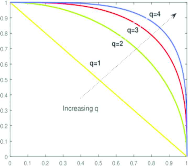
Figure 1

Geometrical interpretation of the intuitionistic fuzzy set (IFS), pythagorean fuzzy set (PYFS), and complex q-rung orthopair fuzzy set (QROFS).

Further, complex IFS (CIFS) was explored by Alkouri and Salleh [23], as a modified notion of the complex FS (CFS) [24], which contains two functions called as truth and falsity grades by the form of complex numbers from unit disc in a complex plane, whose sum of real parts (Also imaginary parts) is not exceeded to the unit interval. CIFS is an effective tool to describe two-dimensional information in a single set, and it has received extensive attention. For example, Ngan et al. [25] represented the CIFS by quaternion numbers; Garg and Rani [26,27] established new generalized Bonferroni mean (BM) operators and robust averaging-geometric operators for CIFS.

However, the scope of the CIFS is narrow because it should satisfy the condition that the sum of the real part (also imaginary part) of truth and the real part (also imaginary part) of the falsity grades is bounded to the unit interval. If some DMs provide such kind of information whose sum of real parts (also imaginary parts) is not limited to the unit interval, CIFS cannot describe it. For example, considering the pair 0.6ei2Π0.61,0.5ei2Π0.51 represents the truth grade and the falsity grade which cannot hold the condition of CIFS 0.6+0.5=1.1≰1 and 0.61+0.51=1.12≰1. Therefore, in order to deal with these issues, Ullah et al. [28] explored complex PYFS (CPYFS), which contains two functions called as truth and falsity grades by the form of complex numbers from unit disc in a complex plane, whose sum of squares in real parts (also imaginary parts) is not exceeded to the unit interval. CPYFS is an effective tool to describe the complicated fuzzy information, and it has received extensive attention. Akram and Naz [29] explored the complex pythagorean fuzzy graphs.

However, the scope of the CPYFS is narrow because it should satisfy the condition that the sum of squares of the real part (Also imaginary part) of truth and the real part (also imaginary part) of the falsity grades is bounded to the unit interval. If some DMs provide such kind of information whose sum of squares in the real part (also imaginary part) of truth and the real part (also imaginary part) is not limited to the unit interval, the CPYFS will not deal with it. For example, considering the pair 0.9ei2Π0.91,0.8ei2Π0.81 represents the truth grade and the falsity grade which cannot hold the condition of CPYFS 0.92+0.82=0.81+0.64=1.45≰1 and 0.912+0.812=0.8281+0.6561=1.4842≰1. Therefore, in order to deal with these issues, complex q-rung orthopair fuzzy set (CQROFFS) was explored by Liu et al. [30,31], which contains two functions called as truth and falsity grades in the form of complex numbers from unit disc in a complex plane, whose sum of q-powers of the real parts (also imaginary parts) is not exceeded to the unit interval. CQROFS is an effective tool to describe the complicated fuzzy information. The comparison of the established work with existing methods [32–36] are also discussed, to examine the reliability and effectiveness of the explored work.

In some real-life decisions, the interrelationships between the attributes are common. For example, in decision-making process of buying a laptop, laptop’s performance and its hardware are related. For taking the responsible decision, it is necessary to choose the interrelationships between the attributes. For coping such kind of problems, the BM operators are playing a key role in examining the interrelationships between the attributes, then Xu and Yager [37] explored the intuitionistic fuzzy BM operators; Liang et al. [38] established the pythagorean fuzzy BM operators and their application in MAGDM. Liu and Liu [32] explored the q-rung orthopair fuzzy BM operators and their application in MAGDM problems. Further, because the constraint of CQROFS is that the sum of q-powers of the real part (also for imaginary part) of the truth and real part (also for imaginary part) of the falsity grades is limited to the unit interval, the CQROFS can provide a wide range to decision information. From the above discussions, it is clear that the CQROFS is more versatile and more superior to CIFS and CPFS to describe awkward and complication information in real-decision. In addition, the BM operators based on CQROFS have not been established yet. So the goals and motivations of this article are explained as follows:

  1. The BM operators based on QROFS [32] is not able to deal with two-dimensional information in a single set. For coping such type of issues, the BM operator based on CQROFS is an important and meaningful concept to examine the interrelationships between the different attributes and can easily cope with two-dimensional information in a single set. So the goals of this article are to establish the complex q-rung orthopair fuzzy BM (CQROFBM) operator, complex q-rung orthopair fuzzy weighted BM (CQROFWBM) operator, complex q-rung orthopair fuzzy geometric BM (CQROFGBM) operator, and complex q-rung orthopair fuzzy weighted geometric BM (CQROFWGBM) operator and to discuss their properties.

  2. Further, we will propose a MAGDM method based on the established operators, which can consider the advantages of BM operators, i.e., considering the interrelationships between the attributes.

  3. Moreover, to examine the feasibility and consistency of the established method, we solve some numerical examples to verify the rationality of the explored operators. The advantages, graphical interpretation, and comparative analysis of the established work are also discussed.

For better understanding, we have drawn the flowchart for the proposed approaches, which is shown in Figure 2.
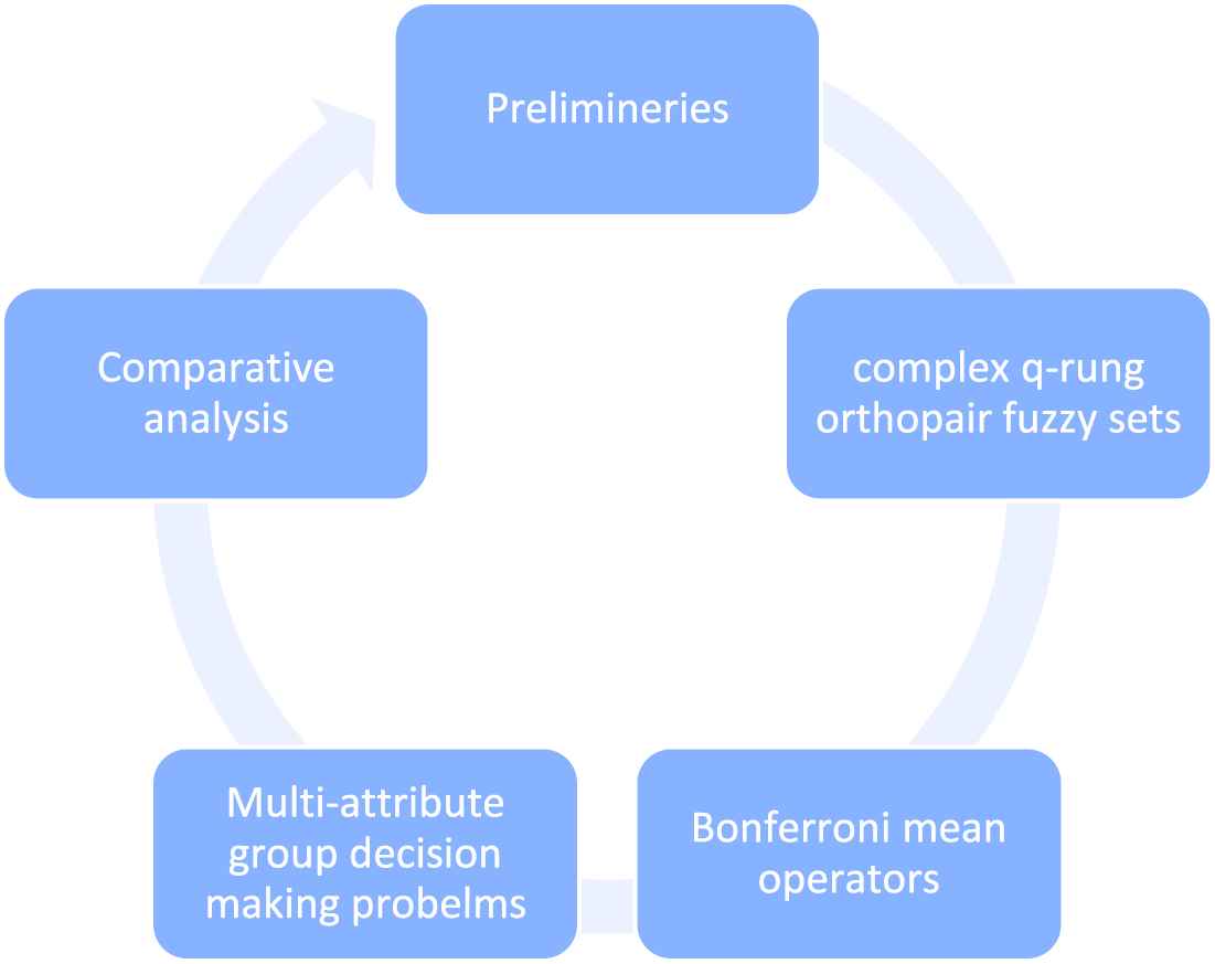
Figure 2

Graphical interpretation of the presented work in this article.

Form Figure 2, it clear that, we propose the BM operator based on CQROFS, which is called complex q-rung orthopair fuzzy BM operator, and discuss its special cases. The proposed technique is more powerful than some other existing operators based on IFS, PFS, QROFS, CIFS, and CPFS. Because the sum of q-powers of the realm parts (also for imaginary parts) of the truth and falsity grades in the CQROFS is not exceeded form unit interval, if we choose the value of parameter q = 1, then the presented work is converted to complex intuitionistic fuzzy BM operator. Similarly if we choose the value of parameter q = 2, then the presented work is converted to complex pythagorean fuzzy BM operator. At the same time, all these operators consider the relationship between two inputs.

The rest of this manuscript is shown as follows: In Section 2, the QROFS, CQROFS, and their operational laws are discussed. In Section 3, the CQROFBM operator, CQROFWBM operator, CQROFGBM operator, and CQROFWGBM operator are explored. In Section 4, we develop the MAGDM method based on the CQROFWGBM operator, and some numerical examples are given to verify the rationality of the explored method. In Section 5, we give the conclusion of this manuscript.

2. PRELIMINARIES

This section is to review some existing notions like QROFSs, CQROFSs, and their operational laws. In this article, we use ŲUnivsersal to represent the fix set. Further, and suppose the symbols keep sCQ,tCQ≥0,qCQ≥1.

Definition 1:

[17] A QROFS is stated by

CQ=𝓊,ΦCQ′𝓊,ξCQ′𝓊:𝓊∈ŲUniversal(1)
where ΦCQ′ and ξCQ′ is called truth and falsity grades with a condition: 0≤ΦCQ′qCQ𝓊+ξCQ′qCQ𝓊≤1. Further, the symbol HCQ𝓊=1−ΦCQ′qCQ𝓊+ξCQ′qCQ𝓊1qCQ represents the hesitancy grade. The q-rung orthopair fuzzy number (QROFN) is denoted by CQ=ΦCQ′𝓊,ξCQ′𝓊.

Definition 2:

[30,31] A CQROFS is stated by

CCQ=𝓊,ΦCCQ′𝓊,ξCCQ′𝓊:𝓊∈ŲUniversal(2)
where ΦCCQ′=ΦCRPei2ΠΨΦCIP and ξCCQ′=ξCRPei2ΠΨξCIP is called truth and falsity grades in the form of complex number from unit disc in a complex plane with conditions 0≤ΦCRPqCQ𝓊+ξCRPqCQ𝓊≤1 and 0≤ΨΦCIPqCQ𝓊+ΨξIPqCQ𝓊≤1. Further, the symbol HCCQ𝓊=μCRPei2ΠΨμCIP=1−ΦCRPqCQ𝓊+ξCRPqCQ𝓊1qCQei2Π1−ΨΦCIPqCQ𝓊+ΨξCIPqCQ𝓊1qCQ represents the hesitancy grade. The complex q-rung orthopair fuzzy number (CQROFN) is denoted by CCQ=ΦCCQ′𝓊,ξCCQ′𝓊=ΦCRPei2ΠΨΦCIP,ξCRPei2ΠΨξCIP.

Definition 3:

[30,31] For any CQROFS CQ=ΦCRPei2ΠΨΦCIP,ξCRPei2ΠΨξCIP, the score function SSF and accuracy function HAF is stated by

SSFCCQ=12ΦCRP−ξCRP+ΨΦCIP−ΨξCIP(3)
HAFCCQ=12ΦCRP+ξCRP+ΨΦCIP+ΨξCIP(4)
where SSFCCQ,HAFCCQ∈−1,1. A comparison between CQROFNs CCQ−1 and CCQ−2 is stated by
  1. If SSFCCQ−1>SSFCCQ−2, then CCQ−1>CCQ−2

  2. If SSFCCQ−1=SSFCCQ−2, then CCQ−1=CCQ−2, then

    1. If HAFCCQ−1>HAFCCQ−2, then CCQ−1>CCQ−2

    2. If HAFCCQ−1=HAFCCQ−2, then CCQ−1=CCQ−2.

Definition 4:

[30,31] For any two CQROFNs CCQ−1 and CCQ−2 with sCQ, the operational laws is stated by

  1. CCQ−1c=ξCRP−1ei2ΠΨξCIP−1,ΦCRP−1ei2ΠΨΦCIP−1

  2. CCQ−1∨CCQ−2=maxΦCRP−1,ΦCRP−2.ei2Π.maxΨΦCIP−1,ΨΦCIP−2,minξCRP−1,ξCRP−2.ei2Π.minΨξCIP−1,ΨξCIP−2

  3. CCQ−1∧CCQ−2=minΦCRP−1,ΦCRP−2.ei2Π.minΨΦCIP−1,ΨΦCIP−2,maxξCRP−1,ξCRP−2.ei2Π.maxΨξCIP−1,ΨξCIP−2

  4. CCQ−1⊕CCQ−2=ΦCRP−1qCQ+ΦCRP−2qCQ−ΦCRP−1qCQΦCRP−2qCQ1qCQ.ei2Π.ΨΦCIP−1qCQ+ΨΦCIP−2qCQ−ΨΦCIP−1qCQΨΦCIP−2qCQ1qCQ,ξCRP−1ξCRP−2.ei2Π.ΨξCIP−1ΨξCIP−2

  5. CCQ−1⊗CCQ−2=ΦCRP−1ΦCRP−2.ei2Π.ΨΦCIP−1ΨΦCIP−2,ξCRP−1qCQ+ξCRP−2qCQ−ξCRP−1qCQξCRP−2qCQ1qCQ.ei2Π.ΨξCIP−1qCQ+ΨξCIP−2qCQ−ΨξCIP−1qCQΨξCRP−2qCQ1qCQ

  6. sCQCCQ−1=1−1−ΦCRP−1qCQsCQ1qCQei2Π.1−1−ΨΦCIP−1qCQsCQ1qCQ,ξCRP−1sCQei2Π.ΨξCIP−1sCQ

  7. CCQ−1sCQ=ΦCRP−1sCQei2Π.ΨΦCIP−1sCQ,1−1−ξCRP−1qCQsCQ1qCQei2Π.1−1−ΨξCRP−1qCQsCQ1qCQ.

Definition 5:

[32] For any non-negative numbers Cj,j=1,2,3,‥,m, we define the BM operators by

 BMsCQ,tCQC1,C2,‥,Cm=1mm−1∑j,k=1j≠kmCjsCQCktCQ1sCQ+tCQ (5)

Definition 6:

[32] For any nonnegative numbers Cj,j=1,2,3,‥,m, we define the GBM operators by

GBMsCQ,tCQ(C1,C2,..,Cm)=1sCQ+tCQ(∏j,k=1j≠km(sCQCj+tCQCk))1m(m−1)(6)

3. BM OPERATORS BASED ON CQROFSs

The purpose of this section is to explore the notions of BM, WBM, geometric BM, and weighted geometric BM operators based on CQROFSs. Further, the special cases of the established operators are also discussed by some remarks.

Definition 7:

For any CQROFN CCQ−j,j=1,2,3,‥,m, we define the CQROFBM operator by

CQROFBMsCQ,tCQCCQ−1,CCQ−2,‥,CCQ−m=1mm−1⊕j,k=1j≠kmCCQ−jsCQ⊗CCQ−ktCQ1sCQ+tCQ(7)

Based on the operational laws in Definition 4 for CQROFBMs, we explore the following results.

Theorem 1:

The aggregation result from Definition 7 is still a CQROFN such that

CQROFBMsCQ,tCQCCQ−1,CCQ−2,‥,CCQ−m=ei2Π1−1−∏j,k=1j≠km2−1−ΨξCIP−jqCQsCQ−1−ΨξCIP−kqCQtCQ−1−1−ΨξCIP−jqCQsCQ1−1−ΨξCIP−kqCQtCQ1mm−11sCQ+tCQ1qCQ.1−∏j,k=1j≠km1−ΦCRP−jsCQΦCRP−ktCQqCQ1mm−11qCQsCQ+tCQ×ei2Π1−∏j,k=1j≠km1−ΨΦCIP−jsCQΨΦCIP−ktCQqCQ1mm−11qCQsCQ+tCQ,1−1−∏j,k=1j≠km2−1−ξCRP−jqCQsCQ−1−ξCRP−kqCQtCQ−1−1−ξCRP−jqCQsCQ1−1−ξCRP−kqCQtCQ1mm−11sCQ+tCQ1qCQ×ei2Π1−1−∏j,k=1j≠km2−1−ΨξCIP−jqCQsCQ−1−ΨξCIP−kqCQtCQ−1−1−ΨξCIP−jqCQsCQ1−1−ΨξCIP−kqCQtCQ1mm−11sCQ+tCQ1qCQ.

Proof:

For any two CQROFNs

CCQ−j=ΦCRP−jei2ΠΨΦCIP−j,ξCRP−jei2ΠΨξCIP−j and CCQ−k=ΦCRP−kei2ΠΨΦCIP−k,ξCRP−kei2ΠΨξCIP−k,
based on Definition 4, we get
CCQ−jsCQ=ΦCRP−jsCQei2ΠΨΦCIP−jsCQ,1−1−ξCRP−jqCQsCQ1qCQei2Π1−1−ΨξCIP−jqCQsCQ1qCQ,
and CCQ−ktCQ=ΦCRP−ktCQei2ΠΨΦCIP−ktCQ,1−1−ξCRP−kqCQtCQ1qCQei2Π1−1−ΨξCIP−kqCQtCQ1qCQ.

Then we have

CCQ−jsCQ⊗CCQ−ktCQ=ΦCRP−jsCQΦCRP−ktCQei2ΠΨΦCIP−jsCQΨΦCIP−ktCQ,2−1−ξCRP−jqCQsCQ−1−ξCRP−kqCQtCQ−1−1−ξCRP−jqCQsCQ1−1−ξCRP−kqCQtCQ1qCQei2Π2−1−ΨξCIP−jqCQsCQ−1−ΨξCIP−kqCQtCQ−1−1−ΨξCIP−jqCQsCQ1−1−ΨξCIP−kqCQtCQ1qCQ
and
∑j,k=1j≠kmCCQ−jsCQ⊗CCQ−ktCQ=1−∏j,k=1j≠km1−ΦCRP−jsCQΦCRP−ktCQqCQ1qCQei2Π1−∏i,j=1i≠jm1−ΨΦCIP−jsCQΨΦCIP−ktCQqCQ1qCQ,∏j,k=1j≠km2−1−ξCRP−jqCQsCQ−1−ξCRP−kqCQtCQ−1−1−ξCRP−jqCQsCQ1−1−ξCRP−kqCQtCQ1qCQei2Π∏j,k=1j≠km2−1−ΨξCIP−jqCQsCQ−1−ΨξCIP−kqCQtCQ−1−1−ΨξCIP−jqCQsCQ1−1−ΨξCIP−kqCQtCQ1qCQ

Further,

1mm−1∑j,k=1j≠kmCCQ−jsCQ⊗CCQ−ktCQ=∏j,k=1j≠km2−1−ξCRP−jqCQsCQ−1−ξCRP−kqCQtCQ−1−1−ξCRP−jqCQsCQ1−1−ξCRP−kqCQtCQ1qCQ1mm−1ei2Π∏j,k=1j≠km2−1−ΨξCIP−jqCQsCQ−1−ΨξCIP−kqCQtCQ−1−1−ΨξCIP−jqCQsCQ1−1−ΨξCIP−kqCQtCQ1qCQ1mm−11−∏j,k=1j≠km1−ΦCRP−jsCQΦCRP−ktCQqCQ1mm−11qCQei2Π1−∏j,k=1j≠km1−ΨΦCIP−jsCQΨΦCIP−ktCQqCQ1mm−11qCQ,∏j,k=1j≠km2−1−ξCRP−jqCQsCQ−1−ξCRP−kqCQtCQ−1−1−ξCRP−jqCQsCQ1−1−ξCRP−kqCQtCQ1qCQ1mm−1ei2Π∏j,k=1j≠km2−1−ΨξCIP−jqCQsCQ−1−ΨξCIP−kqCQtCQ−1−1−ΨξCIP−jqCQsCQ1−1−ΨξCIP−kqCQtCQ1qCQ1mm−1
and
1mm−1⊕j,k=1j≠kmCCQ−jsCQ⊗CCQ−ktCQ1sCQ+tCQ=ei2Π1−1−∏j,k=1j≠km2−1−ΨξCIP−jqCQsCQ−1−ΨξCIP−kqCQtCQ−1−1−ΨξCIP−jqCQsCQ1−1−ΨξCIP−kqCQtCQ1mm−11sCQ+tCQ1qCQ.1−∏j,k=1j≠km1−ΦCRP−jsCQΦCRP−ktCQqCQ1mm−11qCQsCQ+tCQ×ei2Π1−∏j,k=1j≠km1−ΨΦCIP−jsCQΨΦCIP−ktCQqCQ1mm−11qCQsCQ+tCQ,
1−1−∏j,k=1j≠km2−1−ξCRP−jqCQsCQ−1−ξCRP−kqCQtCQ−1−1−ξCRP−jqCQsCQ1−1−ξCRP−kqCQtCQ1mm−11sCQ+tCQ1qCQ×ei2Π1−1−∏j,k=1j≠km2−1−ΨξCIP−jqCQsCQ−1−ΨξCIP−kqCQtCQ−1−1−ΨξCIP−jqCQsCQ1−1−ΨξCIP−kqCQtCQ1mm−11sCQ+tCQ1qCQ.

The proof of the above theorem has been completed.

Further, we explore some properties of CQROFBMsCQ,tCQ operator, including idempotency, monotonicity, and boundedness.

Theorem 2:

For any CQROFN CCQ−j,j=1,2,3,‥,m, then

CQROFBMsCQ,tCQCCQ−1,CCQ−2,‥,CCQ−m=CCQ

Proof:

Suppose CQROFBMsCQ,tCQCCQ−1,CCQ−2,‥,CCQ−m=𝓊,𝓿. We will first prove the membership function, such that ΦCCQ ′=ΦCRPei2ΠΨΦCIP.

Let ΦCRP=ΦCRP−j,ΨΦCIP=ΨΦCIP−j and ΦCRP=ΦCRP−k,ΨΦCIP=ΨΦCIP−k implies that ΦCRPei2ΠΨΦCIP=ΦCRP−jei2ΠΨΦCIP−j and ΦCRPei2ΠΨΦCIP=ΦCRP−kei2ΠΨΦCIP−k, then

𝓊=1−∏j,k=1j≠km1−ΦCRP−jsCQΦCRP−ktCQqCQ1mm−11qCQsCQ+tCQ×ei2Π1−∏j,k=1j≠km1−ΨΦCIP−jsCQΨΦCIP−ktCQqCQ1mm−11qCQsCQ+tCQ=1−∏j,k=1j≠km1−ΦCRP−jsCQΦCRP−ktCQqCQ1mm−11qCQsCQ+tCQ×ei2Π1−∏j,k=1j≠km1−ΨΦCIP−jsCQΨΦCIP−ktCQqCQ1mm−11qCQsCQ+tCQ
=1−∏j,k=1j≠km1−ΦCRPqCQsCQ+tCQ1mm−11qCQsCQ+tCQ×ei2Π1−∏j,k=1j≠km1−ΨΦCIPqCQsCQ+tCQ1mm−11qCQsCQ+tCQ=1−1−ΦCRPqCQsCQ+tCQmm−11mm−11qCQsCQ+tCQ×ei2Π1−1−ΨΦCIPqCQsCQ+tCQmm−11mm−11qCQsCQ+tCQ=1−1+ΦCRPqCQsCQ+tCQ1qCQsCQ+tCQei2Π1−1+ΨΦCIPqCQsCQ+tCQ1qCQsCQ+tCQ=ΦCRPei2ΠΨΦCIP

Based on above approach for truth grade, we also prove falsity grade such that

ξCCQ′=ξCRPei2ΠΨξCIP. Hence

CQROFBMsCQ,tCQCCQ−1,CCQ−2,‥,CCQ−m=CCQ

Theorem 3:

For any two CQROFNs CCQ−j=ΦCRP−jei2ΠΨΦCIP−j,ξCRP−jei2ΠΨξCIP−j and CCQ−∗k=(ΦCRP−∗kei2ΠΨΦCIP−∗k, ξCRP−∗kei2ΠΨξCIP−∗k),(j,k=1,2,..,m), with conditions ΦRP−j≥ΦRP−∗k,ΨΦIP−j≥ΨΦIP−∗k,ξRP−j≤ξRP−∗k and ΨξIP−j≤ΨξIP−∗k, then

CQROFBMsCQ,tCQCCQ−1,CCQ−2,‥,CCQ−m≥CQROFBMsCQ,tCQCCQ−∗1,CCQ−∗2,‥,CCQ−∗m

Proof:

Let CQROFBMsCQ,tCQCCQ−1,CCQ−2,‥,CCQ−m=𝓊,𝓿 and CQROFBMsCQ,tCQCCQ−∗1,CCQ−∗2,‥,CCQ−∗m=𝓊′,𝓿′. The proof of the truth grade, whose real part is as follows: 𝓊′≤𝓊. If Φ∗RP−j≥ΦRP−∗k,Ψ∗ΦIP−j≥ΨΦIP−∗k,ξ∗RP−j≤ξRP−∗k and Ψ∗ξIP−j≤ΨξIP−∗k, then we have

Φ∗RP−jsCQΦ∗RP−∗ktCQei2ΠΨ∗ξIP−jsCQΨ∗ξIP−∗ktCQ≤ΦRP−jsCQΦRP−ktCQei2ΠΨξIP−jsCQΨξIP−ktCQ,
1−Φ∗RP−jsCQΦ∗RP−∗ktCQqCQei2Π1−Ψ∗ξIP−jsCQΨ∗ξIP−∗ktCQqCQ≥1−ΦRP−jsCQΦRP−ktCQqCQei2Π1−ΨξIP−jsCQΨξIP−ktCQqCQ,
∏j,k=1j≠km1−Φ∗RP−jsCQΦ∗RP−∗ktCQqCQ1mm−1ei2Π∏j,k=1j≠km1−Ψ∗ξIP−jsCQΨ∗ξIP−∗ktCQqCQ1mm−1
≥∏j,k=1j≠km1−ΦRP−jsCQΦRP−ktCQqCQ1mm−1ei2Π∏j,k=1j≠km1−ΨξIP−jsCQΨξIP−ktCQqCQ1mm−1
1−∏j,k=1j≠km1−Φ∗RP−jsCQΦ∗RP−∗ktCQqCQ1mm−11qCQsCQ+tCQ×ei2Π1−∏j,k=1j≠km1−Ψ∗ξIP−jsCQΨ∗ξIP−∗ktCQqCQ1mm−11qCQsCQ+tCQ
≤1−∏j,k=1j≠km1−ΦRP−jsCQΦRP−ktCQqCQ1mm−11qCQsCQ+tCQ×ei2Π1−∏j,k=1j≠km1−ΨξIP−jsCQΨξIP−ktCQqCQ1mm−11qCQsCQ+tCQ

Hence 𝓊′≤𝓊. Similarly, 𝓿′≥𝓿, for falsity grade. Thus, the final result is shown as

CQROFBMsCQ,tCQCCQ−1,CCQ−2,‥,CCQ−m≥CQROFBMsCQ,tCQCCQ−∗1,CCQ−∗2,‥,CCQ−∗m.

Theorem 4:

For any two CQROFNs CCQ−j+=maxJΦCRP−jei2ΠmaxJΨΦCIP−j,minjξCRP−jei2ΠminjΨξCIP−j and CCQ−j−=(minJΦCRP−jei2ΠminJΨΦCIP−j,maxjξCRP−jei2ΠmaxjΨξCIP−j),(j=1,2,..,m), then

CCQ−j−≤CQROFBMsCQ,tCQCCQ−1,CCQ−2,‥,CCQ−m≤CCQ−j+

Proof:

Based on monotonicity, we get

CQROFBMsCQ,tCQCCQ−1−,CCQ−2−,‥,CCQ−m−≤CQROFBMsCQ,tCQCCQ−1,CCQ−2,‥,CCQ−m≤CQROFBMsCQ,tCQCCQ−1+,CCQ−2+,‥,CCQ−m+

By idempotency, we get

CQROFBMsCQ,tCQCCQ−1−,CCQ−2−,‥,CCQ−m−=CCQ−j− and CQROFBMsCQ,tCQCCQ−1+,CCQ−2+,‥,CCQ−m+=CCQ−j+

Then

CCQ−j−≤CQROFBMsCQ,tCQCCQ−1,CCQ−2,‥,CCQ−m≤CCQ−j+

The proof of the above theorem has been completed.

Further, the special cases of the  CQROFBMsCQ,tCQ operator are shown as

Remark 1:

When tCQ=0 in Definition 7, then

CQROFBMsCQ,0CCQ−1,CCQ−2,‥,CCQ−m=1−∏j=1m1−ΦCRP−jsCQqCQ1mm−11qCQsCQei2Π1−∏j=1m1−ΨΦCIP−jsCQqCQ1mm−11qCQsCQ,1−1−∏j=1m1−1−ξCRP−jqCQsCQ1mm−11sCQ1qCQ×ei2Π1−1−∏j=1m1−1−ΨξCIP−1qCQsCQ1mm−11sCQ1qCQ

Remark 2:

When sCQ=1,tCQ=0 in Definition 7, then

CQROFBM1,0CCQ−1,CCQ−2,‥,CCQ−m=1−∏j=1m1−ΦCRP−jqCQ1mm−11qCQei2Π1−∏j=1m1−ΨΦCIP−jqCQ1mm−11qCQ,∏j=1mξCRP−jqCQ1qCQmm−1ei2Π∏j=1mΨξCIP−jqCQ1qCQmm−1

Remark 3:

When sCQ=0 in Definition 7, then

CQROFBM0,tCQCCQ−1,CCQ−2,‥,CCQ−m=1−∏k=1m1−ΦCRP−ktCQqCQ1mm−11qCQtCQ×ei2Π1−∏k=1m1−ΨΦCIP−ktCQqCQ1mm−11qCQtCQ,1−1−∏k=1m1−1−ξCRP−kqCQtCQ1mm−11tCQ1qCQ×ei2Π1−1−∏k=1m1−1−ΨξCRP−kqCQsCQ1mm−11tCQ1qCQ

Remark 4:

When sCQ=0,tCQ=1 in Definition 7, then

CQROFBM0,1CCQ−1,CCQ−2,‥,CCQ−m=1−∏k=1m1−ΦCRP−kqCQ1mm−11qCQei2Π1−∏k=1m1−ΨΦCIP−kqCQ1mm−11qCQ,∏k=1mξCRP−kqCQ1qCQmm−1ei2Π∏k=1mΨξCIP−kqCQ1qCQmm−1

Remark 5:

When sCQ=tCQ=1 in Definition 7, then

CQROFBM1,1CCQ−1,CCQ−2,‥,CCQ−m=1−∏j≠k=1m1−ΦCRP−jΦCRP−kqCQ1mm−112qCQei2Π1−∏j≠k=1m1−ΨΦCIP−jΨΦCIP−kqCQ1mm−112qCQ,1−1−∏j≠k=1mξCRP−jqCQ+ξCRP−kqCQ−ξCRP−jqCQξCRP−kqCQ1mm−1121qCQ×ei2Π1−1−∏j≠k=1mΨξCIP−jqCQ+ΨξCIP−kqCQ−ΨξCIP−jqCQΨξCIP−kqCQ1mm−1121qCQ

Further, we define the CQROFWBM operator. Suppose weight vector is Ѡw=Ѡw−1,Ѡw−2,‥,Ѡw−mT,meets∑j=1mѠw−j=1 and Ѡw−j∈0,1,j=1,2,‥,m.

Definition 8:

For any CQROFN CCQ−j,j=1,2,3,‥,m, we define the CQROFWBM operator by

CQROFWBMsCQ,tCQCCQ−1,CCQ−2,‥,CCQ−m=1mm−1⊕j,k=1j≠kmѠw−jCCQ−jsCQ⊗Ѡw−kCCQ−ktCQ1sCQ+tCQ(8)

Based on the operational laws in Definition 4, we give the following results.

Theorem 5:

The aggregation result from Definition 8 is still a CQROFN such that

CQROFWBMsCQ,tCQCCQ−1,CCQ−2,‥,CCQ−m=1−∏j,k=1j≠km1−1−1−ΦCRP−jqCQѠw−jsCQ1−1−ΦCRP−kqCQѠw−ktCQ1mm−11qCQsCQ+tCQ×ei2Π1−∏j,k=1j≠km1−1−1−ΨΦCIP−jqCQѠw−jsCQ1−1−ΨΦCIP−kqCQѠw−ktCQ1mm−11qCQsCQ+tCQ,1−1−∏j,k=1j≠km2−1−ξCRP−jqCQѠw−jsCQ−1−ξCRP−kqCQѠw−ktCQ−1−1−ξCRP−jqCQѠw−jsCQ1−1−ξCRP−kqCQѠw−ktCQ1mm−11sCQ+tCQ1qCQ×ei2Π1−1−∏j,k=1j≠km2−1−ΨξCIP−jqCQѠw−jsCQ−1−ΨξCIP−kqCQѠw−ktCQ−1−1−ΨξCIP−jqCQѠw−jsCQ1−1−ΨξCIP−kqCQѠw−ktCQ1mm−11sCQ+tCQ1qCQ.

Proof:

For any two CQROFNs, it is clear that

Ѡw−jCCQ−j=1−1−ΦCRP−jqCQѠw−j1qCQei2Π1−1−ΨΦCIP−jqCQѠw−j1qCQ,ξCRP−jѠw−jei2ΠΨξCIP−jѠw−j and
Ѡw−kCCQ−k=1−1−ΦCRP−kqCQѠw−k1qCQei2Π1−1−ΨΦCIP−kqCQѠw−k1qCQ,ξCRP−kѠw−kei2ΠΨξCIP−kѠw−k,
then Ѡw−jCCQ−jsCQ=1−1−ΦCRP−jqCQѠw−jsCQqCQei2Π1−1−ΨΦCIP−jqCQѠw−jsCQqCQ,1−1−ξCRP−jqCQѠw−jsCQ1qCQei2Π1−1−ΨξCIP−jqCQѠw−jsCQ1qCQ
and Ѡw−kCCQ−ktCQ=1−1−ΦCRP−kqCQѠw−ktCQqCQei2Π1−1−ΨΦCIP−kqCQѠw−ktCQqCQ,1−1−ξCRP−kqCQѠw−ktCQ1qCQei2Π1−1−ΨξCIP−kqCQѠw−ktCQ1qCQ.

Based on Definition 4, we have

Ѡw−jCCQ−jsCQ⊗Ѡw−kCCQ−ktCQ=1−1−ΦCRP−jqCQѠw−jsCQqCQ1−1−ΦCRP−kqCQѠw−ktCQqCQei2Π1−1−ΨΦCIP−jqCQѠw−jsCQqCQ1−1−ΨΦCIP−kqCQѠw−ktCQqCQ ,2−1−ξCRP−jqCQѠw−jsCQ−1−ξCRP−kqCQѠw−ktCQ−1−1−ξCRP−jqCQѠw−jsCQ1−1−ξCRP−kqCQѠw−ktCQ1qCQei2Π2−1−ΨξCIP−jqCQѠw−jsCQ−1−ΨξCIP−kqCQѠw−ktCQ−1−1−ΨξCIP−jqCQѠw−jsCQ1−1−ΨξCIP−kqCQѠw−ktCQ1qCQ,
and
∑j,k=1j≠kmѠw−jCCQ−jsCQ⊗Ѡw−kCCQ−ktCQ=ei2Π∏j,k=1m2−1−ΨξCIP−jqCQѠw−jsCQ−1−ΨξCIP−kqCQѠw−ktCQ−1−1−ΨξCIP−jqCQѠw−jsCQ1−1−ΨξCIP−kqCQѠw−ktCQ1−∏j,k=1m1−1−ΦCRP−jqCQѠw−jsCQ1−1−ΦCRP−kqCQѠw−ktCQ1qCQei2Π1−∏j,k=1m1−1−ΨΦCIP−jqCQѠw−jsCQ1−1−ΨΦCIP−kqCQѠw−ktCQ1qCQ, ∏j,k=1m2−1−ξCRP−jqCQѠw−jsCQ−1−ξCRP−kqCQѠw−ktCQ−1−1−ξCRP−jqCQѠw−jsCQ1−1−ξCRP−kqCQѠw−ktCQei2Π∏j,k=1m2−1−ΨξCIP−jqCQѠw−jsCQ−1−ΨξCIP−kqCQѠw−ktCQ−1−1−ΨξCIP−jqCQѠw−jsCQ1−1−ΨξCIP−kqCQѠw−ktCQ.

Further,

1mm−1∑j,k=1j≠kmѠw−jCCQ−jsCQ⊗Ѡw−kCCQ−ktCQ=1−∏j,k=1m1−1−ΦCRP−jqCQѠw−jsCQ1−1−ΦCRP−kqCQѠw−ktCQ1mm−11qCQ×ei2Π1−∏j,k=1m1−1−ΨΦCIP−jqCQѠw−jsCQ1−1−ΨΦCIP−kqCQѠw−ktCQ1mm−11qCQ,∏j,k=1m2−1−ξCRP−jqCQѠw−jsCQ−1−ξCRP−kqCQѠw−ktCQ−1−1−ξCRP−jqCQѠw−jsCQ1−1−ξCRP−kqCQѠw−ktCQ1mm+1ei2Π∏j,k=1m2−1−ΨξCIP−jqCQѠw−jsCQ−1−ΨξCIP−kqCQѠw−ktCQ−1−1−ΨξCIP−jqCQѠw−jsCQ1−1−ΨξCIP−kqCQѠw−ktCQ1mm−11mm−1∑j,k=1j≠kmѠw−jCCQ−jsCQ⊗Ѡw−kCCQ−ktCQ1sCQ+tCQ=1−∏j,k=1j≠km1−1−1−ΦCRP−jqCQѠw−jsCQ1−1−ΦCRP−kqCQѠw−ktCQ1mm−11qCQsCQ+tCQ×ei2Π1−∏j,k=1j≠km1−1−1−ΨΦCIP−jqCQѠw−jsCQ1−1−ΨΦCIP−kqCQѠw−ktCQ1mm−11qCQsCQ+tCQ,1−1−∏j,k=1j≠km2−1−ξCRP−jqCQѠw−jsCQ−1−ξCRP−kqCQѠw−ktCQ−1−1−ξCRP−jqCQѠw−jsCQ1−1−ξCRP−kqCQѠw−ktCQ1mm−11sCQ+tCQ1qCQ×ei2Π1−1−∏j,k=1j≠km2−1−ΨξCIP−jqCQѠw−jsCQ−1−ΨξCIP−kqCQѠw−ktCQ−1−1−ΨξCIP−jqCQѠw−jsCQ1−1−ΨξCIP−kqCQѠw−ktCQ1mm−11sCQ+tCQ1qCQ

The proof of the above theorem has been completed.

Further, we explore some properties of the CQROFWBM operator including idempotency, monotonicity, and boundedness.

Theorem 6:

For any CQROFN CCQ−j,j=1,2,3,‥,m, then

CQROFWBMsCQ,tCQCCQ−1,CCQ−2,‥,CCQ−m=CCQ

Proof:

Straightforward.

Theorem 7:

For any two CQROFNs CCQ−j=ΦCRP−jei2ΠΨΦCIP−j,ξCRP−jei2ΠΨξCIP−j and CCQ−∗k=(ΦCRP−∗kei2ΠΨΦCIP−∗k,ξCRP−∗kei2ΠΨξCIP−∗k),(j,k=1,2,..,m), with conditions ΦRP−j≥ΦRP−∗k,ΨΦIP−j≥ΨΦIP−∗k,ξRP−j≤ξRP−∗k and ΨξIP−j≤ΨξIP−∗k, then

CQROFWBMsCQ,tCQCCQ−1,CCQ−2,‥,CCQ−m≥CQROFWBMsCQ,tCQCCQ−∗1,CCQ−∗2,‥,CCQ−∗m

Proof:

Straightforward.

Theorem 8:

For any two CQROFNs CCQ−j+=maxJΦCRP−jei2ΠmaxJΨΦCIP−j,minjξCRP−jei2ΠminjΨξCIP−j and CCQ−j−=(minjΦCRP−jei2ΠminjΨΦCIP−j,maxjξCRP−jei2ΠmaxjΨξCIP−j),(j=1,2,..,m), then

CCQ−j−≤CQROFWBMsCQ,tCQCCQ−1,CCQ−2,‥,CCQ−m≤CCQ−j+

Proof:

According to monotonicity, we get

CQROFWBMsCQ,tCQCCQ−1−,CCQ−2−,‥,CCQ−m−≤CQROFWBMsCQ,tCQCCQ−1,CCQ−2,‥,CCQ−m≤CQROFWBMsCQ,tCQCCQ−1+,CCQ−2+,‥,CCQ−m+

By idempotency, we get

CQROFWBMsCQ,tCQCCQ−1−,CCQ−2−,‥,CCQ−m−=CCQ−j− and CQROFWBMsCQ,tCQCCQ−1+,CCQ−2+,‥,CCQ−m+=CCQ−j+

Then

CCQ−j−≤CQROFWBMsCQ,tCQCCQ−1,CCQ−2,‥,CCQ−m≤CCQ−j+.

The proof of the above theorem has been completed.

Definition 9:

For any CQROFN CCQ−j,j=1,2,3,‥,m, we define the CQROFGBM operator by

CQROFGBMsCQ,tCQCCQ−1,CCQ−2,‥,CCQ−m=1sCQ+tCQ⊗j,k=1j≠kmsCQCCQ−j⊕tCQCCQ−k1mm−1(9)

Based on the operational laws in Definition 4, we give the following result.

Theorem 9:

The aggregation result of the CQROFGBMsCQ,tCQ operator is still a CQROFN such that

CQROFGBMsCQ,tCQCCQ−1,CCQ−2,‥,CCQ−m=1−1−∏j,k=1j≠km2−1−ΦCRP−jqCQsCQ−1−ΦCRP−kqCQtCQ−1−1−ΦCRP−jqCQsCQ1−1−ΦCRP−kqCQtCQ1mm−11sCQ+tCQ1qCQ×ei2Π1−1−∏j,k=1j≠km2−1−ΨΦCIP−jqCQsCQ−1−ΨΦCIP−kqCQtCQ−1−1−ΨΦCIP−jqCQsCQ1−1−ΨΦCIP−kqCQtCQ1mm−11sCQ+tCQ1qCQ,1−∏j,k=1j≠km1−ξCRP−jsCQξCRP−ktCQqCQ1mm−11qCQsCQ+tCQei2Π1−∏j,k=1j≠km1−ΨξCIP−jsCQΨξCIP−ktCQqCQ1mm−11qCQsCQ+tCQ

Proof:

Straightforward.

Further, we explore some properties of the CQROFGBMsCQ,tCQ operator, such as idempotency, monotonicity, and boundedness.

Theorem 10:

For any CQROFN CCQ−j,j=1,2,3,‥,m, then

CQROFGBMsCQ,tCQCCQ−1,CCQ−2,‥,CCQ−m=CCQ.

Proof:

Straightforward.

Theorem 11:

For any two CQROFNs CCQ−j=ΦCRP−jei2ΠΨΦCIP−j,ξCRP−jei2ΠΨξCIP−j and CCQ−∗k=(ΦCRP−∗kei2ΠΨΦCIP−∗k,ξCRP−∗kei2ΠΨξCIP−∗k),(j,k=1,2,..,m), with conditions ΦRP−j≥ΦRP−∗k,ΨΦIP−j≥ΨΦIP−∗k,ξRP−j≤ξRP−∗k and ΨξIP−j≤ΨξIP−∗k, then

CQROFGBMsCQ,tCQCCQ−1,CCQ−2,‥,CCQ−m≥CQROFGBMsCQ,tCQCCQ−∗1,CCQ−∗2,‥,CCQ−∗m

Proof:

Straightforward.

Theorem 12:

For any two CQROFNs CCQ−j+=maxJΦCRP−jei2ΠmaxJΨΦCIP−j,minjξCRP−jei2ΠminjΨξCIP−j and CCQ−j−=(minJΦCRP−jei2ΠminJΨΦCIP−j,maxjξCRP−jei2ΠmaxjΨξCIP−j),(j=1,2,..,m), then

CCQ−j−≤CQROFGBMsCQ,tCQCCQ−1,CCQ−2,‥,CCQ−m≤CCQ−j+.

Proof:

According to monotonicity, we get

CQROFGBMsCQ,tCQCCQ−1−,CCQ−2−,‥,CCQ−m−≤CQROFGBMsCQ,tCQCCQ−1,CCQ−2,‥,CCQ−m≤CQROFGBMsCQ,tCQCCQ−1+,CCQ−2+,‥,CCQ−m+

By idempotency, we get

CQROFGBMsCQ,tCQCCQ−1−,CCQ−2−,‥,CCQ−m−=CCQ−j− and CQROFGBMsCQ,tCQCCQ−1+,CCQ−2+,‥,CCQ−m+=CCQ−j+

Then

CCQ−j−≤CQROFGBMsCQ,tCQCCQ−1,CCQ−2,‥,CCQ−m≤CCQ−j+.

The proof of the above theorem has been completed.

Further, the special cases of the CQROFGBMsCQ,tCQ operator are shown as

Remark 6:

When tCQ=0 in Definition 9, then

CQROFWGBMsCQ,0(CCQ−1,CCQ−2,‥,CCQ−m)=1−1−∏j,k=1j≠km1−1−ΦCRP−jqCQsCQ1mm−11sCQ1qCQ×ei2Π1−1−∏j,k=1j≠km1−1−ΨΦCIP−jqCQsCQ1mm−11sCQ1qCQ,1−∏j,k=1j≠km1−ξCRP−jsCQqCQ1mm−11qCQsCQ×ei2Π1−∏j,k=1j≠km1−ΨξCIP−jsCQqCQ1mm−11qCQsCQ.

Remark 7:

When sCQ=1,tCQ=0 in Definition 9, then

CQROFWGBM1,0CCQ−1,CCQ−2,‥,CCQ−m=1−1−∏j,k=1j≠kmΦCRP−jqCQ1mm−111qCQei2Π1−1−∏j,k=1j≠kmΨΦCIP−jqCQ1mm−111qCQ,1−∏j,k=1j≠km1−ξCRP−j 1qCQ1mm−11qCQei2Π1−∏j,k=1j≠km1−ΨξCIP−j 1qCQ1mm−11qCQ.

Remark 8:

When sCQ=0 in Definition 9, then

CQROFGBM0,tCQCCQ−1,CCQ−2,‥,CCQ−m=1−1−∏j,k=1j≠km1−1−ΦCRP−jqCQtCQ1mm−11tCQ1qCQei2Π1−1−∏j,k=1j≠km1−1−ΨΦCIP−jqCQtCQ1mm−11tCQ1qCQ1−∏j,k=1j≠km1−ξCRP−jtCQqCQ1mm−11qCQtCQei2Π1−∏j,k=1j≠km1−ΨξCIP−jtCQqCQ1mm−11qCQtCQ.

Remark 9:

When sCQ=0,tCQ=1 in Definition 9, then

CQROFGBM0,1CCQ−1,CCQ−2,‥,CCQ−m=1−1−∏j,k=1j≠kmΦCRP−jqCQ1mm−111qCQei2Π1−1−∏j,k=1j≠kmΨΦCIP−jqCQ1mm−111qCQ,1−∏j,k=1j≠km1−ξCRP−j 1qCQ1mm−11qCQei2Π1−∏j,k=1j≠km1−ΨξCIP−j 1qCQ1mm−11qCQ.

Remark 10:

When sCQ=tCQ=1 in Definition 9, then

CQROFGBM1,1CCQ−1,CCQ−2,‥,CCQ−m=1−1−∏j,k=1j≠kmΦCRP−jqCQ+ΦCRP−kqCQ−ΦCRP−jqCQΦCRP−kqCQ1mm−1121qCQ×ei2Π1−1−∏j,k=1j≠kmΨΦCIP−jqCQ+ΨΦCIP−kqCQ−ΨΦCIP−jqCQΨΦCIP−kqCQ1mm−1121qCQ,1−∏j,k=1j≠km1−ξCRP−jξCRP−kqCQ1mm−112qCQei2Π1−∏j,k=1j≠km1−ΨξCIP−jΨξCIP−kqCQ1mm−112qCQ.

Further, we explore the CQROFWGBM operator. Suppose the weight vector is stated by Ѡw=Ѡw−1,Ѡw−2,‥,Ѡw−mT,∑j=1mѠw−j=1 and Ѡw−j∈0,1,j=1,2,‥,m.

Definition 10:

For any CQROFN CCQ−j,j=1,2,3,‥,m, we define the CQROFWGBM operator by

CQROFWGBMsCQ,tCQCCQ−1,CCQ−2,‥,CCQ−m=1sCQ+tCQ⊗j,k=1j≠kmsCQCCQ−jѠw−j⊕tCQCCQ−kѠw−k1mm−1(10)

Based on the operational laws in Definition 4, we give the following result.

Theorem 13:

The aggregation result of CQROFWGBMsCQ,tCQ operator is still a CQROFN such that

CQROFWGBMsCQ,tCQCCQ−1,CCQ−2,‥,CCQ−m=1−1−∏j,k=1j≠km2−1−ΦCRP−jqCQѠw−jsCQ−1−ΦCRP−kqCQѠw−ktCQ−1−1−ΦCRP−jqCQѠw−jsCQ1−1−ΦCRP−kqCQѠw−ktCQ1mm−11sCQ+tCQ1qCQ×ei2Π1−1−∏j,k=1j≠km2−1−ΨΦCIP−jqCQѠw−jsCQ−1−ΨΦCIP−kqCQѠw−ktCQ−1−1−ΨΦCIP−jqCQѠw−jsCQ1−1−ΨΦCIP−kqCQѠw−ktCQ1mm−11sCQ+tCQ1qCQ,1−∏j,k=1j≠km1−1−1−ξCRP−jqCQѠw−jsCQ1−1−ξCRP−kqCQѠw−ktCQ1mm−11qCQsCQ+tCQ×ei2Π1−∏j,k=1j≠km1−1−1−ΨξCIP−jqCQѠw−jsCQ1−1−ΨξCIP−kqCQѠw−ktCQ1mm−11qCQsCQ+tCQ.

Proof:

Straightforward.

Further, we explore some properties of CQROFWGBMsCQ,tCQ operator, such as idempotency, monotonicity, and boundedness.

Theorem 14:

For any CQROFN CCQ−j,j=1,2,3,‥,m, then

CQROFWGBMsCQ,tCQCCQ−1,CCQ−2,‥,CCQ−m=CCQ.

Proof:

Straightforward.

Theorem 15:

For any two CQROFNs CCQ−j=ΦCRP−jei2ΠΨΦCIP−j,ξCRP−jei2ΠΨξCIP−j and CCQ−∗k=ΦCRP−∗kei2ΠΨΦCIP−∗k,ξCRP−∗kei2ΠΨξCIP−∗k,j,k=1,2,‥,m, with conditions ΦRP−j≥ΦRP−∗k,ΨΦIP−j≥ΨΦIP−∗k,ξRP−j≤ξRP−∗k and ΨξIP−j≤ΨξIP−∗k, then

CQROFWGBMsCQ,tCQCCQ−1,CCQ−2,‥,CCQ−m≥CQROFWGBMsCQ,tCQCCQ−∗1,CCQ−∗2,‥,CCQ−∗m.

Proof:

Straightforward.

Theorem 16:

For any two CQROFNs CCQ−j+=maxJΦCRP−jei2ΠmaxJΨΦCIP−j,minjξCRP−jei2ΠminjΨξCIP−j and CCQ−j−=minJΦCRP−jei2ΠminJΨΦCIP−j,maxjξCRP−jei2ΠmaxjΨξCIP−j,j=1,2,‥,m, then

CCQ−j−≤CQROFWGBMsCQ,tCQCCQ−1,CCQ−2,‥,CCQ−m≤CCQ−j+

Proof:

Based on monotonicity, we get

CQROFWGBMsCQ,tCQCCQ−1−,CCQ−2−,‥,CCQ−m−≤CQROFWGBMsCQ,tCQCCQ−1,CCQ−2,‥,CCQ−m≤CQROFWGBMsCQ,tCQCCQ−1+,CCQ−2+,‥,CCQ−m+

By idempotency, we get

CQROFWGBMsCQ,tCQCCQ−1−,CCQ−2−,‥,CCQ−m−=CCQ−j− and CQROFWGBMsCQ,tCQCCQ−1+,CCQ−2+,‥,CCQ−m+=CCQ−j+

Then

CCQ−j−≤CQROFWGBMsCQ,tCQCCQ−1,CCQ−2,‥,CCQ−m≤CCQ−j+.

The proof of the above theorem has been completed.

4. MULTI-ATTRIBUTE GROUP DECISION MAGDM METHOD BASED ON ESTABLISHED OPERATORS

The purpose of this section is to utilize the established operators to solve the MAGDM problems.

4.1. Description of MAGDM Problems

The purpose of the MAGDM Problems is to select the best one from the family of alternatives. Suppose D=D1,D2,‥,Dt,Ų=Ų1,Ų2,‥,Ųm and A=A1,A2,‥,An respectively represent the families of DMs, alternatives and their attributes. Moreover, we use the CQROFN CCQ−jk p=ΦCRP−jk pei2ΠΨΦCIP−jk p,ξCRP−jk pei2ΠΨξCIP−jk p to express the evaluation value of the alternative Ųj under the attribute Ap given by the DM Dk, then get the matrices Ap=Cjk pm×n. The weight vector of experts is ℧w−j=℧w−1,℧w−2,‥,℧w−tT,∑j=1t℧w−j=1 and ℧w−i∈0,1,j=1,2,‥,t and the weight vector of attributes is Ѡw−j=Ѡw−1,Ѡw−2,‥,Ѡw−nT,∑j=1nѠw−j=1 and Ѡw−j∈0,1,j=1,2,‥,n. Based on the above data, the steps of the algorithm are stated by

4.2. Procedure of the Algorithm

  1. Based on Subsection 4.1, we give the decision matrix.

    rjk p=CCQ−jk p,C′CQ−jk p=ΦCRP−jk pei2ΠΨΦCIP−jk p,ξCRP−jk pei2ΠΨξCIP−jk pfor benefitξCRP−jk pei2ΠΨξCIP−jk p,ΦCRP−jk pei2ΠΨΦCIP−jk pfor cost(11)

  2. Based on Eq. (12), we can obtain the comprehensive value of each alternative from each DM

    rj p=Cjk p,C′jk p=CQROFWBMsCQ,tCQCCQ−j1 p,CCQ−j2 p,‥,CCQ−jn p(12)

  3. Based on Eq. (13), we can get the comprehensive value of each alternative.

    rj p=Cj,k p,C′j,k p=CQROFWGBMsCQ,tCQCCQ−j1 p,CCQ−j2 p,‥,CCQ−jn p(13)

  4. Based on score function, we calculate the score functions of above aggregated values.

  5. Rank the score values and examine the best one.

  6. The end.

For more clarity, we make flowchart for the above algorithm which is shown in Figure 3.
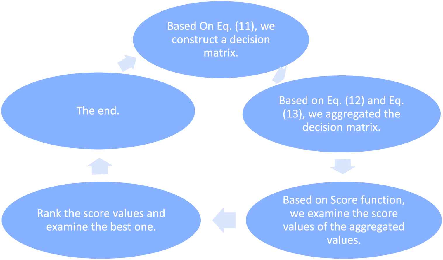
Figure 3

Graphical interpretation for the procedure of the algorithm of 4.2.

4.3. Illustrated Numerical Examples

The purpose of this section is to show the reliability and proficiency of the proposed method by some numerical examples.

Example 1:

To examine the feasibility and validity of the explored method in this manuscript, we use an investment problem to explain it. In order to select one suitable investment alternative from five companies Ų=Ų1,Ų2,‥,Ų5 which are explained as follows:

  • Ų1 is a car company

  • Ų2 is a laptop company

  • Ų3 is a mobile company

  • Ų4 is a food company

  • Ų5 is a furniture company

Further, these companies are evaluated by four attributes A=A1,A2,‥,A4, which are explained in Table 1, and three experts D=D1,D2,D3 give the evaluation information stated in Tables 2–4. Moreover, the weight vector of experts is ℧w−3=0.5,0.35,0.15T and the weight vector of attributes is Ѡw−4=0.35,0.22,0.29,0.14T. The goal is to give a best choice for investment.

A1 A2 A3 A4
Risk analysis Growth analysis Social-political impact analysis Environmental impact analysis
Table 1

Information about attributes and their representations.

Data Representation A1 A2 A3 A4
Ų1 (0.6ei2Π0.6,0.5ei2Π0.54) (0.67ei2Π0.76,0.78ei2Π0.8) (0.76ei2Π0.87,0.83ei2Π0.74) (0.58ei2Π0.89,0.87ei2Π0.77)
Ų2 (0.8ei2Π0.67,0.77ei2Π0.85) (0.7ei2Π0.67,0.81ei2Π0.85) (0.67ei2Π0.55,0.8ei2Π0.9) (0.67ei2Π0.56,0.8ei2Π0.87)
Ų3 (0.86ei2Π0.78,0.7ei2Π0.65) (0.73ei2Π0.68,0.82ei2Π0.86) (0.68ei2Π0.66,0.78ei2Π0.89) (0.56ei2Π0.45,0.88ei2Π0.9)
Ų4 (0.82ei2Π0.76,0.72ei2Π0.86) (0.6ei2Π0.69,0.9ei2Π0.87) (0.57ei2Π0.78,0.8ei2Π0.79) (0.77ei2Π0.55,0.89ei2Π0.91)
Ų5 (0.86ei2Π0.72,0.73ei2Π0.8) (0.67ei2Π0.7,0.84ei2Π0.88) (0.59ei2Π0.54,0.88ei2Π0.87) (0.6ei2Π0.56,0.93ei2Π0.92)
Table 2

Complex q-rung orthopair fuzzy decision matrix Z1 given by D1.

Data Representation A1 A2 A3 A4
Ų1 (0.78ei2Π0.76,0.67ei2Π0.54) (0.76ei2Π0.87,0.83ei2Π0.74) (0.76ei2Π0.89,0.87ei2Π0.77) (0.87ei2Π0.83,0.74ei2Π0.76)
Ų2 (0.81ei2Π0.67,0.7ei2Π0.85) (0.67ei2Π0.55,0.8ei2Π0.9) (0.67ei2Π0.56,0.8ei2Π0.87) (0.55ei2Π0.8,0.9ei2Π0.67)
Ų3 (0.82ei2Π0.68,0.73ei2Π0.65) (0.68ei2Π0.66,0.78ei2Π0.89) (0.68ei2Π0.45,0.88ei2Π0.9) (0.66ei2Π0.78,0.89ei2Π0.68)
Ų4 (0.9ei2Π0.69,0.6ei2Π0.86) (0.57ei2Π0.78,0.8ei2Π0.79) (0.57ei2Π0.55,0.89ei2Π0.91) (0.78ei2Π0.8,0.79ei2Π0.57)
Ų5 (0.84ei2Π0.7,0.67ei2Π0.8) (0.59ei2Π0.54,0.88ei2Π0.87) (0.59ei2Π0.56,0.93ei2Π0.92) (0.54ei2Π0.88,0.87ei2Π0.59)
Table 3

Complex q-rung orthopair fuzzy decision matrix Z2 given by D2.

Data Representation A1 A2 A3 A4
Ų1 (0.87ei2Π0.76,0.54ei2Π0.83) (0.5ei2Π0.6,0.6ei2Π0.77) (0.87ei2Π0.83,0.8ei2Π0.76) (0.87ei2Π0.78,0.74ei2Π0.87)
Ų2 (0.85ei2Π0.67,0.55ei2Π0.8) (0.8ei2Π0.67,0.77ei2Π0.87) (0.55ei2Π0.8,0.85ei2Π0.67) (0.55ei2Π0.8,0.9ei2Π0.8)
Ų3 (0.65ei2Π0.68,0.64ei2Π0.78) (0.7ei2Π0.78,0.86ei2Π0.67) (0.66ei2Π0.78,0.86ei2Π0.68) (0.66ei2Π0.78,0.89ei2Π0.88)
Ų4 (0.86ei2Π0.57,0.78ei2Π0.8) (0.72ei2Π0.76,0.82ei2Π0.89) (0.78ei2Π0.8,0.87ei2Π0.57) (0.78ei2Π0.7,0.79ei2Π0.89)
Ų5 (0.8ei2Π0.59,0.54ei2Π0.88) (0.73ei2Π0.72,0.86ei2Π0.92) (0.54ei2Π0.88,0.88ei2Π0.59) (0.54ei2Π0.56,0.87ei2Π0.89)
Table 4

Complex q-rung orthopair fuzzy decision matrix Z3 given by D3.

For solving this kind of decision problems, the presented approach is better than existing approaches based on the structure of the CQROFS. The CQROFS meets a condition that the sum of q-powers of the real parts (also for imaginary parts) of the truth and falsity grades is not exceeded form unit interval, and it is more general than QROFS, PFS, CPFS, IFS, CIFS, and etc. Because the BM operators are more generalized than various existing operators like weighted averaging, weighted geometric based on some existing notion like QROFS, PFS, CPFS, IFS, CIFS, and etc. Keeping the advantages of the BM operator based on CQROFS, we solve this problem to check the reliability and effectiveness of the explored method.

The decision procedure is shown as follows:

  1. Based on Eq. (11), we get the normalized decision matrix. The measured information is same, which is not necessary to require the normalization.

  2. Based on Eq. (12), we obtain the comprehensive value of each alternative from each DM (suppose qCQ=4,sCQ=tCQ=1)

    r1 1=0.05ei2Π0.12,0.85ei2Π0.76. r2 1=0.07ei2Π0.04,0.88ei2Π0.87.

    r3 1=0.08ei2Π0.06,0.88ei2Π0.86. r4 1=0.07ei2Π0.08,0.90ei2Π0.87.

    r5 1=0.07ei2Π0.05,0.91ei2Π0.88. r12=0.11ei2Π0.16,0.88ei2Π0.75.

    r22=0.07ei2Π0.05,0.88ei2Π0.80. r32=0.08ei2Π0.05,0.90ei2Π0.79.

    r42=0.08ei2Π0.07,0.87ei2Π0.78. r52=0.06ei2Π0.06,0.92ei2Π0.79.

    r13=0.14ei2Π0.09,0.80ei2Π0.84. r23=0.08ei2Π0.08,0.87ei2Π0.81.

    r33=0.05ei2Π0.09,0.90ei2Π0.84. r43=0.12ei2Π0.07,0.90ei2Π0.84.

    r53=0.06ei2Π0.08,0.89ei2Π0.86.

  3. Based on Eq. (13), we get the comprehensive value of each alternative (qCQ=4,sCQ=tCQ=1).

    r1=0.14ei2Π0.15,0.21ei2Π0.13. r2=0.09ei2Π0.08,0.25ei2Π0.18.

    r3=0.08ei2Π0.08,0.26ei2Π0.17. r4=0.12ei2Π0.09,0.26ei2Π0.19.

    r5=0.08ei2Π0.08,0.30ei2Π0.20.

  4. Based on score function, we calculate the score functions of above aggregated values.

    Sr1=−0.00064, Sr2=−0.002333, Sr3=−0.00287, Sr4=−0.00293, Sr5=−0.00465.

  5. Rank the score values and examine the best one company for investment.

    Ų1≥Ų2≥Ų3≥Ų4≥Ų5

  6. Consequently, Ų1 is the best one in the above five companies, which is car company.

  7. End.

Now we can compare the established method with existing methods in expressing the different fuzzy information, and the results are shown in Table 5.

Methods Score Function Ranking Best Alternatives
Garg and Rani [33] Cannot be calculated Cannot be calculated No
Rani and Garg [34] Cannot be calculated Cannot be calculated No
CPYFS for qCQ=2 in this article Cannot be calculated Cannot be calculated No
Cq-ROFS proposed in this article Sr1=−0.00064, Sr2=−0.002333, Sr3=−0.00287, Sr4=−0.00293, Sr5=−0.00465. Ų1≥Ų2≥Ų3≥Ų4≥Ų5 Ų1
Table 5

Comparison method between the proposed and existing methods.

4.4. Influence on Decision Results for the Different Parameters

The parameters in the developed operators play a key role in the final ranking results. In order to show their influence on decision results, the ranking results for the different parameters are shown in the Tables 6–8.

Parameters Score Values Ranking
sCQ=tCQ=1 Sr1=0.177, Sr2=0.114, Sr3=0.110, Sr4=0.126, Sr5=0.095. Ų1≥Ų2≥Ų4≥Ų3≥Ų5
sCQ=2,tCQ=1 Sr1=0.223, Sr2=0.171, Sr3=0.174,Sr4=0.186, Sr5=0.163. Ų1≥Ų4≥Ų3≥Ų2≥Ų5
sCQ=5,tCQ=1 Sr1=0.186, Sr2=0.147, Sr3=0.152,Sr4=0.161, Sr5=0.145. Ų1≥Ų4≥Ų3≥Ų1≥Ų5
sCQ=10,tCQ=1 Sr1=0.143, Sr2=0.117, Sr3=0.123,Sr4=0.128, Sr5=0.116. Ų1≥Ų4≥Ų3≥Ų2≥Ų5
sCQ=15,tCQ=1 Sr1=0.118, Sr2=0.099, Sr3=0.105,Sr4=0.109, Sr5=0.098. Ų1≥Ų4≥Ų3≥Ų2≥Ų5
sCQ=20,tCQ=1 Sr1=0.100, Sr2=0.088, Sr3=0.093,Sr4=0.095, Sr5=0.087. Ų1≥Ų4≥Ų3≥Ų2≥Ų5
Table 6

Ranking values for constant parameter t = 1 and variable parameter s.

Parameters Score Values Ranking
sCQ=tCQ=1 Sr1=0.177, Sr2=0.114, Sr3=0.110,Sr4=0.126, Sr5=0.095. Ų1≥Ų2≥Ų4≥Ų3≥Ų5
sCQ=1,tCQ=2 Sr1=0.226, Sr2=0.173, Sr3=0.176,Sr4=0.189, Sr5=0.167. Ų1≥Ų4≥Ų3≥Ų2≥Ų5
sCQ=1,tCQ=5 Sr1=0.196, Sr2=0.147, Sr3=0.154,Sr4=0.164, Sr5=0.145. Ų1≥Ų4≥Ų3≥Ų1≥Ų5
sCQ=1,tCQ=10 Sr1=0.166, Sr2=0.126, Sr3=0.133,Sr4=0.140, Sr5=0.124. Ų1≥Ų4≥Ų3≥Ų2≥Ų5
sCQ=1,tCQ=15 Sr1=0.146, Sr2=0.113, Sr3=0.121, Sr4=0.126, Sr5=0.112. Ų1≥Ų4≥Ų3≥Ų2≥Ų5
sCQ=1,tCQ=20 Sr1=0.133, Sr2=0.104, Sr3=0.112,Sr4=0.117, Sr5=0.104. Ų1≥Ų4≥Ų3≥Ų2≥Ų5
Table 7

Ranking values for constant parameter s = 1 and variable parameter t.

Parameters Score Values Ranking
qCQ=3 Sr1=−0.014, Sr2=−0.019, Sr3=−0.022, Sr4=−0.021, Sr5=−0.026. Ų1≥Ų2≥Ų4≥Ų3≥Ų5
qCQ=5 Sr1=−0.0046, Sr2=−0.0073, Sr3=−0.0089, Sr4=−0.0088, Sr5=−0.012. Ų1≥Ų2≥Ų4≥Ų3≥Ų5
qCQ=8 Sr1=−0.0013, Sr2=−0.0023, Sr3=−0.00302, Sr4=−0.003, Sr5=−0.004. Ų1≥Ų2≥Ų4≥Ų3≥Ų5
qCQ=10 Sr1=−0.0005, Sr2=−0.0012, Sr3=−0.0016, Sr4=−0.0016, Sr5=−0.025. Ų1≥Ų2≥Ų4≥Ų3≥Ų5
qCQ=15 Sr1=−0.0000000098, Sr2=−0.00026, Sr3=−0.00039, Sr4=−0.00039, Sr5=−0.00072. Ų1≥Ų2≥Ų4≥Ų3≥Ų5
Table 8

Ranking values for parameter q.

From Tables 6 and 7, we can know these ranking results are changed for the different values of parameters. However, the best one is still Ų1.

From Table 8, it is shown the developed operators based on CQROFS is more general then existing notions due to its constraint, i.e., the sum of q-powers of the real part (also for imaginary part) of the truth and the falsity grades is not exceed from unit interval.

4.5. Comparison of the Established Operators with Some Existing Operators

The explored operators based on CQROFS in this paper is more general than some existing operators due to its constraint, i.e., the sum of q-powers of the real part (also for imaginary part) of the truth and the falsity grades is not exceed from unit interval. Based on comparison between the established method with existing ones, we examine the advantages and superiority of the explored work which is shown in Table 9.

Aggregation Operators Operator Capture the Interrelation between the Cq-ROFNs A Parameter Vector Exists to Manipulate the Ranking Results Contain Two-Dimension Information
q-ROFWA [35] No No No
q-ROFWG [35] No No No
q-ROFHM [36] Yes Yes No
q-ROFWHM [36] Yes Yes No
q-ROFBM [32] Yes Yes No
q-ROFWBM [32] Yes Yes No
q-ROFGBM [32] Yes Yes No
q-ROFWGBM [32] Yes Yes No
Cq-ROFBM Yes Yes Yes
Cq-ROFWBM Yes Yes Yes
Cq-ROFGBM Yes Yes Yes
Cq-ROFWGBM Yes Yes Yes

Note: q-ROFWA, q-rung orthopair weighted averaging; q-ROFWG, q-rung orthopair fuzzy weighted geometric; q-ROFHM, q-rung orthopair fuzzy Heronian mean; q-ROFWHM, q-rung orthopair fuzzy weighted Heronian mean; q-ROFBM, q-rung orthopair fuzzy Bonferroni mean; q-ROFWBM, q-rung orthopair fuzzy weighted Bonferroni mean; q-ROFGBM, q-rung orthopair fuzzy geometric Bonferroni mean; q-ROFWGBM, q-rung orthopair fuzzy weighted geometric Bonferroni mean; Cq-ROFBM, complex q-rung orthopair fuzzy Bonferroni mean; Cq-ROFWBM, complex q-rung orthopair fuzzy weighted Bonferroni mean; Cq-ROFGBM, complex q-rung orthopair fuzzy geometric Bonferroni mean; Cq-ROFWGBM, complex q-rung orthopair fuzzy weighted geometric Bonferroni mean.

Table 9

Characteristic comparison between the proposed method and existing methods.

From Table 9, it is clear that the existing operators in [32] are not able to evaluate our considered kinds of information in the form of two-dimension in a single set, and the established operators in this paper are more valuable than existing operators.

To moreover examine the superiority of the explored approach in the MADM environment, we solve a numerical example based on established operator and also for existing operators to show the effectiveness of the explored work. The existing methods were established by Garg and Rani [33], Rani and Garg [34], and Liu et al. [30,31] with different kinds of aggregation operators established for CIFSs and CQROFSs.

Example 2:

The information related to this example is given in Example 1. We consider complex pythagorean kinds of information and evaluated the validity and reliability of the established operators in this manuscript, we solve a numerical example whose information is shown in Table 10 and the weight vector of the attributes is Ѡw−4=0.35,0.22,0.29,0.14T.

Data Representation A1 A2 A3 A4
Ų1 (0.6ei2Π0.6,(0.5)ei2Π(0.54)) (0.67ei2Π0.24,(0.28)ei2Π(0.22)) (0.6ei2Π0.5,(0.43)ei2Π(0.24)) (0.58ei2Π0.5,(0.47)ei2Π(0.17))
Ų2 (0.4ei2Π0.67,(0.6)ei2Π(0.3)) (0.7ei2Π0.33,(0.31)ei2Π(0.21)) (0.67ei2Π0.55,(0.28)ei2Π(0.25)) (0.67ei2Π0.5,(0.38)ei2Π(0.07))
Ų3 (0.86ei2Π0.3,(0.24)ei2Π(0.4)) (0.73ei2Π0.23,(0.32)ei2Π(0.23)) (0.68ei2Π0.5,(0.28)ei2Π(0.3)) (0.56ei2Π0.45,(0.37)ei2Π(0.19))
Ų4 (0.8ei2Π0.3,(0.22)ei2Π(0.24)) (0.6ei2Π0.6,(0.5)ei2Π(0.11)) (0.57ei2Π0.5,(0.5)ei2Π(0.21)) (0.77ei2Π0.25,(0.29)ei2Π(0.11))
Ų5 (0.86ei2Π0.22,(0.13)ei2Π(0.24)) (0.67ei2Π0.5,(0.34)ei2Π(0.19)) (0.59ei2Π0.5,(0.51)ei2Π(0.2)) (0.6ei2Π0.5,(0.43)ei2Π(0.12))
Table 10

Complex pythagorean fuzzy decision matrix for Example 2

The evaluated results are listed in Table 11.

Methods Score Function Ranking
Garg and Rani [33] Cannot be calculated Cannot be calculated
Rani and Garg [34] Cannot be calculated Cannot be calculated
Cq-ROFBM proposed in this article qCQ=2 Sr1=−0.416, Sr2=−0.375, Sr3=−0.351, Sr4=−0.342, Sr5=−0.337. Ų5≥Ų4≥Ų3≥Ų2≥Ų1
Cq-ROFBM proposed in this article qCQ=3 Sr1=−0.193, Sr2=−0.158, Sr3=−0.130, Sr4=−0.139, Sr5=−0.130. Ų5≥Ų3≥Ų4≥Ų2≥Ų1
Table 11

Comparison methods between the proposed and existing methods from Example 2

From Table 11, we can see that the proposed method is better than the existing ones in expressing the fuzzy information.

Example 3:

The information related to this example is given in Example 1. We consider complex intuitionistic kinds of information and evaluated the validity and reliability of the established operators in this manuscript, we solve a numerical example whose information is shown in Table 12 and the weight vector of the attributes is Ѡw−4=0.35,0.22,0.29,0.14T.

Data Representation A1 A2 A3 A4
Ų1 (0.4ei2Π0.3,(0.5)ei2Π(0.54)) (0.7ei2Π0.24,(0.28)ei2Π(0.22)) (0.36ei2Π0.5,(0.43)ei2Π(0.24)) (0.58ei2Π0.5,(0.27)ei2Π(0.17))
Ų2 (0.4ei2Π0.6,(0.6)ei2Π(0.3)) (0.57ei2Π0.33,(0.31)ei2Π(0.21)) (0.37ei2Π0.55,(0.28)ei2Π(0.25)) (0.67ei2Π0.5,(0.18)ei2Π(0.07))
Ų3 (0.6ei2Π0.3,(0.24)ei2Π(0.4)) (0.53ei2Π0.23,(0.32)ei2Π(0.23)) (0.38ei2Π0.5,(0.28)ei2Π(0.3)) (0.56ei2Π0.45,(0.17)ei2Π(0.19))
Ų4 (0.45ei2Π0.3,(0.22)ei2Π(0.24)) (0.36ei2Π0.6,(0.5)ei2Π(0.11)) (0.37ei2Π0.5,(0.5)ei2Π(0.21)) (0.77ei2Π0.25,(0.19)ei2Π(0.11))
Ų5 (0.56ei2Π0.22,(0.13)ei2Π(0.24)) (0.37ei2Π0.5,(0.34)ei2Π(0.19)) (0.39ei2Π0.5,(0.51)ei2Π(0.2)) (0.6ei2Π0.5,(0.23)ei2Π(0.12))
Table 12

Complex intuitionistic fuzzy decision matrix for Example 3

The evaluated results are listed in Table 13.

Methods Score Function Ranking
Garg and Rani [33] Sr1=−0.570, Sr2=−0.557, Sr3=−0.534, Sr4=−0.547, Sr5=−0.533. Ų5≥Ų4≥Ų3≥Ų2≥Ų1
Rani and Garg [34] Sr1=−0.704, Sr2=−0.672, Sr3=−0.667, Sr4=−0.658, Sr5=−0.651. Ų5≥Ų4≥Ų3≥Ų2≥Ų1
Cq-ROFBM proposed in this article qCQ=2 Sr1=−0.397, Sr2=−0.350, Sr3=−0.328, Sr4=−0.328, Sr5=−0.315. Ų5≥Ų4≥Ų3≥Ų2≥Ų1
Cq-ROFBM proposed in this article qCQ=3 Sr1=−0.171, Sr2=−0.133, Sr3=−0.111, Sr4=−0.125, Sr5=−0.109. Ų5≥Ų3≥Ų4≥Ų2≥Ų1
Table 13

Comparison methods between the proposed and existing methods from Example 3

From Table 13, it is clear that the all existing operators in [32] are able to evaluate our considered kinds of information for qCQ=1, and they are a special case of the proposed operators.

To give a large space for expressing the fuzzy information and to consider the relationship between attributes, we established some BM operators using CQROFSs. It is clear that the CIFS and CPYFS are a special case of the established CQROFSs. When we set qCQ=1, then the CQROFS is reduced to CIFS, and similarly when we set qCQ=2, then it is reduced to CPYFS. Hence the established operators based on CQROFS are more powerful and more efficient than some existing operators due to its condition and its parameters.

5. CONCLUSION

Recently, Liu et al. [30,31] explored the novel approach of CQROFS, which is the mixture of the two notions like QROFS and CFS. The CIFS and CPFS are a good tool to the express the fuzzy information. However, CQROFS is more general, to cope with awkward and complicated information due to its outstanding feature that the sum of q-powers of the real part (also for imaginary part) of the truth and real part (also for imaginary part) of the falsity grades is limited to the unit interval. BM operator is an important and meaningful concept to examine the interrelationships between the different attributes. The aims of this manuscript explored the CQROFBM operator, CQROFWBM operator, CQROFGBM operator, and CQROFWGBM operator, and proposed the decision-making method based on the developed operators. Finally, we have used the practical cases to illustrate the feasibility and superiority of the proposed method by comparative analysis with the other existing methods.

In the future, we will extend the proposed approach to the different environment and then apply to the fields of the similarity measures, aggregation operators [39–46].

DATA AVAILABILITY

The data used to support the findings of this study are included within the article.

CONFLICT OF INTEREST

The authors declare that there are no conflict of interest regarding the publication of this article.

AUTHORS' CONTRIBUTION

All authors contributed equally.

ACKNOWLEDGMENTS

This paper is supported by the National Natural Science Foundation of China (Nos. 71771140 and 71471172), 文化名家暨“四个一批”人才项目 (Project of cultural masters and “the four kinds of a batch” talents) and the Special Funds of Taishan Scholars Project of Shandong Province (No. ts201511045).

REFERENCES

46.N. Jan, Z. Ali, T. Mahmood, and K. Ullah, Some generalized distance and similarity measures for picture hesitant fuzzy sets and their applications in building material recognition and multi-attribute decision making, Punjab Univ. J. Math., Vol. 51, 2019, pp. 51-70.
Journal
International Journal of Computational Intelligence Systems
Volume-Issue
13 - 1
Pages
822 - 851
Publication Date
2020/06/22
ISSN (Online)
1875-6883
ISSN (Print)
1875-6891
DOI
10.2991/ijcis.d.200514.001How to use a DOI?
Copyright
© 2020 The Authors. Published by Atlantis Press SARL.
Open Access
This is an open access article distributed under the CC BY-NC 4.0 license (http://creativecommons.org/licenses/by-nc/4.0/).

Cite this article

TY  - JOUR
AU  - Peide Liu
AU  - Zeeshan Ali
AU  - Tahir Mahmood
AU  - Nasruddin Hassan
PY  - 2020
DA  - 2020/06/22
TI  - Group Decision-Making Using Complex q-Rung Orthopair Fuzzy Bonferroni Mean
JO  - International Journal of Computational Intelligence Systems
SP  - 822
EP  - 851
VL  - 13
IS  - 1
SN  - 1875-6883
UR  - https://doi.org/10.2991/ijcis.d.200514.001
DO  - 10.2991/ijcis.d.200514.001
ID  - Liu2020
ER  -