On Relationship between L-valued Approximation Spaces and L-valued Transformation Systems

Sutapa Mahato; S.P. Tiwari

doi:10.2991/ijcis.d.200904.001

<Previous Article In Issue

Download article (PDF)

Next Article In Issue>

Volume 13, Issue 1, 2020, Pages 1464 - 1472

On Relationship between L-valued Approximation Spaces and L-valued Transformation Systems

Authors

Sutapa Mahato, S.P. Tiwari^*

Department of Mathematics and Computing, Indian Institute of Technology (ISM), Dhanbad-826004, India

^*Corresponding author. Email: sptiwarimaths@gmail.com

Corresponding Author

S.P. Tiwari

Received 9 May 2020, Accepted 2 September 2020, Available Online 14 September 2020.

DOI: 10.2991/ijcis.d.200904.001 How to use a DOI?
Keywords: L-valued approximation spaces; L-valued natural transformation; L-valued transformation systems; Category; Functor
Abstract: The objective of this paper is to establish the relationship between L-valued approximation spaces and L-valued transformation systems. We show that for each L-valued upper/lower fuzzy transformation system there exist an L-valued reflexive approximation space and vice versa. In between, we study the concept of L-valued natural transformations.
Copyright: © 2020 The Authors. Published by Atlantis Press B.V.
Open Access: This is an open access article distributed under the CC BY-NC 4.0 license (http://creativecommons.org/licenses/by-nc/4.0/).

1. INTRODUCTION

The concept of rough set was originally proposed by Pawlak [1]. This theory has been developed significantly due to its importance for the study of intelligent systems with insufficient and incomplete information. In rough sets introduced by Pawlak, the key role is played by equivalence relations. In literature [2–4], several generalizations of rough sets have been made by replacing the equivalence relation by an arbitrary relation. Further, Dubois and Prade [5] introduced the concept of fuzzy rough set, in which fuzzy relations play a key role instead of crisp relations. Recently, the combinations of fuzzy sets and rough sets were investigated with different fuzzy logic operations and binary fuzzy relation in [6–14], where fuzzy implications play an important role in the extensions of fuzzy rough sets. In a recent study, Li and Yue established more general model of fuzzy rough sets based on L-valued relation. They investigated it from both constructive and axiomatic approaches, where L is a GL-quantale. In this model of fuzzy rough sets, the key components are a universal set A (as an L-set), an L- valued equivalence relation on A and an L-subset of A (cf., [15], for details).

Fuzzy transform (F-transform in short), firstly proposed by Perfilieva [16], has now been significantly developed and opened a new page in the theory of semi-linear spaces. It was shown in [16] that this transform encompassed both classical transform as well as approximation methods based on fuzzy IF-THEN rules studied in fuzzy modeling. The theory of F-transform was further elaborated and extended from real valued to lattice valued functions [16,17] and from fuzzy sets to parametrized fuzzy sets [18]. Recently in [19], it is shown that F-transform is a realization of an abstract fuzzy rough set theory, more precisely, F-transforms turn out to be fuzzy approximation operators. In another direction, the concepts of upper and lower fuzzy transformation systems were introduced recently by Močkoř [20] and a close connection with F-transforms was established. Specifically, it was shown that a function satisfies axioms for fuzzy upper (or lower, respectively) transformation systems if and only if it is an upper (or lower, respectively) F-transform.

In view of the facts that (i) an F-transform can be viewed as a fuzzy approximation operator and (ii) there is a bijective correspondence between an F-transform and a fuzzy transformation system, it is natural to think about the relationship between a fuzzy approximation operator and a fuzzy transformation system. In this work, we have established such relationship, where fuzzy approximation operators are considered as studied in [15].

The paper is organized as follows: In Section 2, we recall some basic properties of residuated lattice, MV-algebra and L-valued relation. The concept of L-valued approximation spaces and their properties are discussed in Section 3. In Section 4, the relationship between L-valued upper natural transformation and L-valued lower natural transformation is discussed. In Section 5, we study a relationship between L-valued transformation systems and L-valued reflexive approximation spaces. At last, we conclude our research in Section 6.

2. PRELIMINARIES

In this section, we recall some basic notions of residuated lattices, MV-algebra and L-valued relations. For details on residuated lattices and MV-algebra, we refer the works done in [21–24,15,25–27]. We begin with the following:

Definition 2.1.

A residuated lattice is an algebra L≡(L,∧,∨,⊗,→,0,1) such that

(L,∧,∨,0,1) is a bounded lattice with the least element 0 and the greatest element 1;
(L,⊗,1) is a commutative monoid; and
∀a,b,c∈L; a⊗b≤c iff a≤b→c, i.e., (→,⊗) is an adjoint pair on L.

A residuated lattice (L,∧,∨,⊗,→,0,1) is complete if it is complete as a lattice.

Proposition 2.1

Let L≡(L,∧,∨,⊗,→,0,1) be a residuated lattice. Then for a,b,c,bi∈L, we have

a→1=1, 1→a=a,
a≤b⇒a→b=1,
a≤b⇒a⊗c≤b⊗c, a→c≥b→c, c→a≤c→b,
a⊗0=0, a⊗1=a,
a→(b→c)=b→(a→c),
a→∨i∈Ibi≥∨i∈I(a→bi),
a⊗∨i∈Ibi=∨i∈I(a⊗bi),
a→∧i∈Ibi=∧i∈I(a→bi).

Definition 2.2

Let L≡(L,∧,∨,⊗,→,0,1) be a residuated lattice. Then L is said to be divisible if for a,b∈L and a≤b, ∃c∈L such that a=b⊗c. Further, it is said to satisfy idempotency if a⊗a=a. A negation in L is a unary operation ¬ defined by ¬a=a→0, ∀a∈L. L is said to satisfy the law of double negation if ¬(¬a)=a, for all a∈L. An MV-algebra is a residuated lattice satisfies both divisibility and double negation law.

Proposition 2.2

Let L≡(L,∧,∨,⊗,→,0,1) be an MV-algebra. Then for a,b,c∈L, we have

a⊗(a→b)=a∧b,
ifa≤b, then b∧[(b→a)→c]=b⊗(a→c),
if a,c≤b, then c⊗(b→a)=a⊗(b→c),
a→b=¬(a⊗¬b),
¬a→¬b=b→a,
if a⊗a=a, then a∧b=a⊗b.

Throughout the paper, unless otherwise stated, L is a complete residuated lattice. For a nonempty set A0, an L-set A of A0 is defined as a mapping from A0 to L. Let B:A0→L be an L-set and B(x)≤A(x),x∈A0. Then the mapping B is called an L-subset of A. The family of all L-subsets of A is denoted by PA. For any a∈L, a is a constant L-subset of A defined by a(x)=a if a≤A(x) and a(x)=0 otherwise. For any B,C∈PA, the union, intersection, ⊗-intersection and →-implication of B and C are defined as L-subsets of A by (B∨C)(x)=B(x)∨C(x); (B∧C)(x)=B(x)∧C(x); (B⊗C)(x)=B(x)⊗C(x); (B→C)(x)=B(x)→C(x). Further, let A:A0→L be an L-set. Then for y∈A0, two new L-sets Ay and A−y0 are defined by

Ay(x)=A(x),if x=y,0,if x≠y,A−y0(x)=A(x),if x≠y,0,if x=y.

Obviously, Ay and A−y0 are L-subsets of A. Furthermore, for all B∈PA, core(B) is a set of all elements x∈A0 such that B(x)=A(x).

Now, we recall the following from [15].

Definition 2.3

Let A:A0→L and B:B0→L be two L-sets. An L-valued relation P is a mapping P:A0×B0→L such that P(x,y)≤A(x)∧B(y),∀x∈A0,y∈B0.

Definition 2.4

Let A be an L-set and let P:A0×A0→L be an L-valued relation on A. Then P is called

reflexive if P(x,x)=A(x), for all x∈A0;
transitive if P(x,y)⊗(A(y)→P(y,z))≤P(x,z), for all x,y,z∈A0; and
symmetric if P(x,y)=P(y,x), for all x,y∈A0.

A reflexive, transitive and symmetric L-valued relation on A is called an L-valued equivalence relation on A.

In above definition, if we take A=1X, then P is an L-fuzzy relation. Thus an L-fuzzy relation is a special case of an L-valued relation.

Definition 2.5

Let P be an L-valued equivalence relation on A. For x∈A0, an L-subset ExP of A such that ExP(y)=P(x,y), for y∈A0, is called an L-valued equivalence class of P determined by the element x.

3. L-VALUED APPROXIMATION SPACES

In this section, we study the concept of L-valued approximation spaces. Further, it is shown that the L-valued lower approximation operator preserves union under certain condition. Now, we recall the following from [15]:

Definition 3.1

Let A:A0→L be an L-set and P be an L-valued relation on A. The pair (A,P) is called an L-valued approximation space. The operators PA¯, PA̲:PA→PA are respectively called the L-valued upper and L-valued lower approximation operator of (A,P) where for all B∈PA and all x∈A0,

PA¯(B)(x)=∨y∈A0B(y)⊗(A(y)→P(y,x))

PA̲(B)(x)=∧y∈A0A(x)⊗(P(y,x)→B(y)).

The pair (PA¯(B),PA̲(B)) is called an L-valued rough set of B with respect to (A,P).

Remark 3.1.

In above definition, if we take A=1X, then L-valued upper approximation operator and L-valued lower approximation operator are consistent with L-fuzzy upper approximation operator and L-fuzzy lower approximation operator, respectively, studied in [26].

Let L be an MV-algebra. Then according to Proposition 2.2, the L-valued lower rough approximation operator PA̲ can be expressed as follows:

PA̲(B)(x)=∧y∈A0A(x)∧[(A(x)→P(y,x))→B(y)].

Now, we have the following.

Proposition 3.1

Let (A,P) be an L-valued approximation space. Then for all B,C∈PA,

PA̲(B∨C)≥PA̲(B)∨PA̲(C).

Proof:

For x∈A0,

PA̲(B∨C)(x)=∧y∈A0A(x)⊗(P(y,x)→(B∨C)(y))≥∧y∈A0[A(x)⊗{(P(y,x)→(B)(y))∨(P(y,x)→(C)(y))}],[from Proposition 2.1(8)]≥∧y∈A0[{A(x)⊗(P(y,x)→(B)(y))}∨{A(x)⊗(P(y,x)→(C)(y))}],[from Proposition 2.1(9)]≥{∧y∈A0{A(x)⊗(P(y,x)→(B)(y))}}∨{∧y∈A0{A(x)⊗(P(y,x)→(C)(y))}}≥PA̲(B)(x)∨PA̲(C)(x)≥(PA̲(B)∨PA̲(C))(x).

PA̲(B∨C)≥(PA̲(B)∨PA̲(C)).

In an L-valued approximation space (A,P), for B,C∈PA, PA̲(B∨C)≠PA̲(B)∨PA̲(C), which is shown as under (cf., [28]).

Counter-Example 3.1.

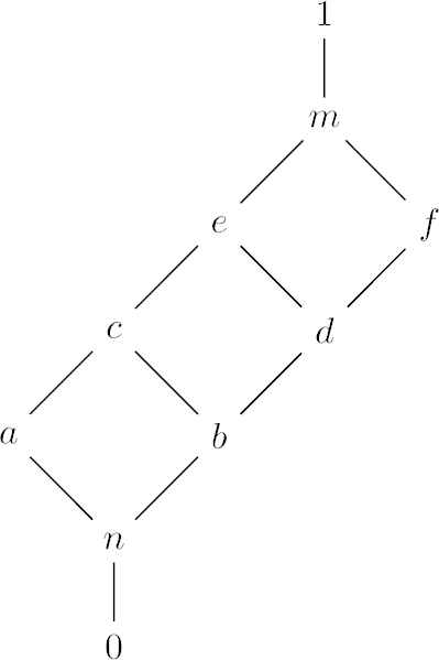
Let L={0,n,a,b,c,d,e,f,m,1} with 0<n<a<c<e<m<1, 0<n<b<d<f<m<1 and the elements {a,b}, {c,d},{e,f} are pairwise incomparable. Then L becomes a residuated lattice to the operations shown in Tables 1 and 2. Hasse diagram of residuated lattice L is given Figure 1.

→	0	n	a	b	c	d	e	f	m	1
0	1	1	1	1	1	1	1	1	1	1
n	m	1	1	1	1	1	1	1	1	1
a	f	f	1	f	1	f	1	f	1	1
b	e	e	e	1	1	1	1	1	1	1
c	d	d	e	f	1	f	1	f	1	1
d	c	c	c	e	e	1	1	1	1	1
e	b	b	c	d	e	f	1	f	1	1
f	a	a	a	c	c	e	e	1	1	1
m	n	n	a	b	c	d	e	f	1	1
1	0	n	a	b	c	d	e	f	m	1

Table 1

→ operation for lattice L.

⊗	n	a	b	c	d	e	f	m	1
0	0	0	0	0	0	0	0	0	0
n	0	0	0	0	0	0	0	0	n
a	0	a	0	a	0	a	0	a	a
b	0	0	0	0	0	0	b	b	b
c	0	a	0	a	0	a	b	c	c
d	0	0	0	0	b	b	d	d	d
e	0	a	0	a	b	c	d	e	e
f	0	0	b	b	d	d	f	f	f
m	0	a	b	c	d	e	f	m	m
1	n	a	b	c	d	e	f	m	1

Table 2

⊗ operation for lattice L.

Let A={(x,1),(y,1),(z,1)} and B, C be two L-subsets of A such that B={(x,b),(y,c),(z,d)}, C={(x,b),(y,d),(z,d)}. Then B∨C={(x,b),(y,e),(z,d)}, since c∨d=e. Now, let P be an L-valued relation on A, as given in Table 3. Then

PA̲(B∨C)(x)=∧y∈A0A(x)⊗{P(y,x)→(B∨C)(y)} =(b→b)∧(e→e)∧(d→d) =1∧1∧1 =1.

P	x	y	z
x	b	o	e
y	e	b	m
z	d	f	1

Table 3

Fuzzy binary relation on X.

Also,

PA̲(B)(x)=∧y∈A0A(x)⊗{P(y,x)→(B)(y)} =(b→b)∧(e→c)∧(d→d) =1∧e∧1 =e.

And

PA̲(C)(x)=∧y∈A0A(x)⊗{P(y,x)→(C)(y)} =(b→b)∧(e→d)∧(d→d) =1∧f∧1 =f.

But, e∨f=m≠1. Hence PA̲(B∨C)≠PA̲(B)∨PA̲(C).

Following is toward the condition under which equality holds.

Proposition 3.2

Let (A,P) be an L-valued approximation space and B,C∈PA. Then PA̲(B∨C)=(PA̲(B)∨PA̲(C)), if ∣ExP∣=1, for every x∈A0.

Proof:

If ∣ExP∣=1 for x∈A0. Then

P(x,y)=A(x)if x=y0if x≠y

Now, for x∈A0,

PA̲(B∨C)(x)=∧y∈A0{A(x)⊗(P(y,x)→(B∨C)(y))}=[∧x=y∈A0{A(x)⊗(A(x)→(B∨C)(y))}]∧[∧x≠y∈A0{A(x)⊗(0→(B∨C)(y))}]=[∧x=y∈A0{(B∨C)(y)}]∧[∧x≠y∈A0{A(x)⊗1}],[from Proposition 2.1(1,4)]=(B∨C)(x)=B(x)∨C(x).

Again, for x∈A0,

PA̲(B)(x)=∧y∈A0A(x)⊗(P(y,x)→B(y))=[∧x=y∈A0{A(x)⊗(A(x)→B(y))}]∧[∧x≠y∈A0{A(x)⊗(0→B(y))}]=[∧x=y∈A0B(y)]∧[∧x≠y∈A0{A(x)⊗1}],[from Proposition 2.1(1,4)]=B(x).

Similarly, we can show that, PA̲(C)(x)=C(x). Thus from above PA̲(B∨C)(x)=PA̲(B)(x)∨PA̲(C)(x). Hence PA̲(B∨C)=PA̲(B)∨PA̲(C).

4. L-VALUED NATURAL TRANSFORMATIONS

In this section, we introduce the concepts of L-valued lower and upper backward natural transformations. Further, we show that there is a close connection between such transformations and maps between two L-valued approximation spaces.

Throughout the rest part of this paper, A10,A20 are two nonempty sets and A1,A2 are L-sets of A10 and A20, respectively. The following is a concept of L-valued Zadeh's backward operator.

Definition 4.1

Let A10 and A20 be two nonempty sets. Again let A1 and A2 be L-sets of A10 and A20, respectively and ϕ:A10→A20 be a map. Then L-valued Zadeh's backward operator ϕ←:PA2→PA1 is defined as follows:

ϕ←(B2)(x1)=B2(ϕ(x1))⊗A1(x1),∀B2∈PA2,∀x1∈A10.

Definition 4.2

Let (A1,P1) and (A2,P2) be two L-valued approximation spaces. A one-one map ϕ:A10→A20 is called

An L-valued upper backward natural transformation from (A1,P1) to (A2,P2), if P1¯(ϕ←(B2))≤ϕ←(P2¯(B2)), ∀B2∈PA2, and
An L-valued relation preserving map if A2(ϕ(y1))⊗P1(y1,x1)≤P2(ϕ(y1),ϕ(x1))⊗A1(x1).

Now, we have the following:

Proposition 4.1

Let L be an MV algebra, (A1,P1), (A2,P2) be two L-valued approximation spaces and ϕ:A10→A20 be a one-one map. Then ϕ is an L-valued upper backward natural transformation if and only if ϕ is L-valued relation preserving map provided L satisfies idempotency property.

Proof:

Let ϕ be an L-valued relation preserving map. Then P2(ϕ(y1),ϕ(x1))⊗A1(x1)≥A2(ϕ(y1))⊗P1(y1,x1). Again, let ϕ(y1)=y2. Then for B2∈PA2,

A2(ϕ(y1))⊗P1(y1,x1)≤P2(ϕ(y1),ϕ(x1))⊗A1(x1)B2(ϕ(y1))⊗P1(y1,x1)≤A1(x1)⊗P2(ϕ(y1),ϕ(x1)),[from Proposition 2.1(3)]{B2(ϕ(y1))⊗B2(ϕ(y1))}⊗P1(y1,x1)≤B2(ϕ(y1))⊗A1(x1)⊗P2(ϕ(y1),ϕ(x1))B2(ϕ(y1))⊗A1(y1)⊗{A1(y1)→P1(y1,x1d)}≤B2(ϕ(y1))⊗A1(x1)⊗{A2(y2)→P2(ϕ(y1),ϕ(x1))}, [from Proposition 2.1(3) and Proposition 2.2(1)]∨y1∈A10[ϕ←(B2)(y1)⊗{A1(y1)→P1(y1,x1)}]≤∨y2∈A20[B2(y2)⊗{A2(y2)→P2(y2,ϕ(x1))}]⊗A1(x1)P1¯(ϕ←(B2))(x1)≤P2¯(B2)(ϕ(x1))⊗A1(x1)P1¯∘ϕ←(B2)(x1)≤ϕ←∘P2¯(B2)(x1)P1¯∘ϕ←≤ϕ←∘P2¯.

Thus ϕ is an L-valued upper backward natural transformation. Conversely, let ϕ be an L-valued upper backward natural transformation. Then

P1¯∘ϕ←(A2y2)(x1)=∨z1∈A10{ϕ←(A2y2)(z1)⊗{A1(z1)→P1(z1,x1)}}=∨z1∈A10[{A2y2(ϕ(z1))⊗A1(z1)}⊗{A1(z1)→P1(z1,x1)}]=∨z1∈A10[A2y2(ϕ(z1))⊗{A1(z1)⊗{A1(z1)→P1(z1,x1)}}]=∨z1∈A10{A2y2(ϕ(z1))⊗P1(z1,x1)}=A2(y2)⊗P1(y1,x1).

Now,

ϕ←∘P2¯(A2y2)(x1)=P2¯(A2y2)(ϕ(x1))⊗A1(x1)=∨z2∈A20[A2y2(z2)⊗{A2(z2)→P2(z2,ϕ(x1)}]⊗A1(x1)=A2(y2)⊗{A2(y2)→P2(y2,ϕ(x1)}⊗A1(x1)=P2(y2,ϕ(x1))⊗A1(x1).

Also,

ϕ←∘P2¯≥P1¯∘ϕ← ϕ←∘P2¯(A2y2)(x1)≥P1¯∘ϕ←(A2y2)(x1) P2(y2,ϕ(x1))⊗A1(x1)≥A2(y2)⊗P1(y1,x1) P2(ϕ(y1),ϕ(x1))⊗A1(x1)≥A2(ϕ(y1))⊗P1(y1,x1).

Thus ϕ is an L-valued relation preserving map.

Definition 4.3

Let (A1,P1) and (A2,P2) be two L-valued approximation spaces. A one-one map ϕ:A10→A20 is called an L-valued lower backward natural transformation from (A1,P1) to (A2,P2), if P1̲(ϕ←(B2))≥ϕ←(P2̲(B2)), ∀B2∈PA2.

Before stating next, we recall the following from [15]:

Definition 4.4

Let L be an MV-algebra. Then the pseudo complement of B∈PA is defined as follows:

∼B(x)=A(x)⊗(¬B(x)), ∀x∈A0.

Proposition 4.2

Let (A,P) be an L-valued approximation space and let PA¯ and PA̲ be L-valued upper and L-valued lower approximation operators of (A,P). Then for all B∈PA,

∼PA¯(∼B)=PA̲(B),

∼PA̲(∼B)=PA¯(B)

Proposition 4.3

Let L be an MV-algebra. Then

For all B∈PA, ∼(∼B)=B,
If B≤C, then ∼B≥∼C, ∀B,C∈PA.

Proof:

(i) For all B∈PA and x∈A0,

∼(∼B)(x)=A(x)⊗(∼B(x)→0) =A(x)⊗{(A(x)⊗¬B(x))→0} =A(x)⊗¬{(A(x)⊗¬B(x))} =A(x)⊗(A(x)→B(x)),[from Proposition 2.2(4)] =B(x),[from Proposition 2.2(1)].

Hence the proof.

(ii) Let B≤C. Then B(x)≤C(x), or ¬B(x)≥¬C(x), or A(x)⊗(¬B(x))≥A(x)⊗(¬C(x)), or that ∼B(x)≥∼C(x), ∀x∈A0.

Lemma 4.1

Let L be an MV-algebra and let (A1,P1) and (A2,P2) be two L-valued approximation spaces. A one-one map ϕ:A10→A20 is an L-valued upper backward natural transformation if and only if ϕ is L-valued lower backward natural transformation provided L satisfies idempotency property and A1(x1)≤A2(ϕ(x1)), ∀x1∈A10.

Proof:

For B2∈PA2 and x1∈A10,

∼ϕ←(B2)(x1)=A1(x1)⊗¬ϕ←(B2)(x1) =A1(x1)⊗¬(B2(ϕ(x1))⊗A1(x1)) =A1(x1)⊗{A1(x1)→¬(B2(ϕ(x1)))} =A1(x1)∧¬(B2(ϕ(x1))),[from Proposition 2.2(1)] =A1(x1)⊗¬(B2(ϕ(x1))),[from Proposition 2.2(6)].

Again,

ϕ←(∼B2)(x1)=∼B2(ϕ(x1))⊗A1(x1) ={A2(ϕ(x1))⊗¬B2(ϕ(x1))}⊗A1(x1) ={A2(ϕ(x1))⊗A1(x1)}⊗¬B2(ϕ(x1)) ={A2(ϕ(x1))∧A1(x1)}⊗¬B2(ϕ(x1)) =A1(x1)⊗¬B2(ϕ(x1)).

Thus ∼ϕ←(B2)(x1)=ϕ←(∼B2)(x1). Now,

ϕ←(P2¯(B2))≥P1¯(ϕ←(B2)) ⇔∼ϕ←(P2¯(B2))≤∼P1¯(ϕ←(B2)) ⇔ϕ←(∼P2¯(B2))≤P1̲(∼ϕ←(B2)) ⇔ϕ←(P2̲(∼B2))≤P1̲(ϕ←(∼B2)).

Replacing ∼B2 by B2, we have ϕ←(P2̲(B2))≤P1̲(ϕ←(B2)). Hence ϕ is an L-valued lower backward natural transformation.

Finally, we have the following:

Proposition 4.4

Let L be an MV-algebra and (A1,P1), (A2,P2) be two L-valued approximation spaces. A one-one map ϕ:A10→A20 is an L-valued lower backward natural transformation if and only if ϕ is L-valued relation preserving map provided L satisfies idempotency property and A1(x1)≤A2(ϕ(x1)), ∀x1∈A10.

Proof:

Follows from the Proposition 4.1 and Lemma 4.1.

5. L-VALUED TRANSFORMATION SYSTEMS VERSUS L-VALUED APPROXIMATION SPACES

In this section, we introduce and study the concepts of L-valued upper/lower transformation systems. Interestingly, we show that there is bijection between L-valued upper/lower transformation systems and L-valued reflexive approximation spaces. We begin with the following:

Definition 5.1

Let G:PA→PA be a map. Then the system (A,G) is called an L-valued upper transformation system if

For each B∈PA, B(x)≤G(B)(x),
For each {Bi:i∈I}∈PA, G(∨i∈IBi)=∨i∈IG(Bi),
For each a,b∈L with a≤b and ∨x∈A0B(x)≤b, G(a⊗(b→B))=a⊗(b→G(B)),
Core (G(Ay))≠∅.

Lemma 5.1

Let B∈PA. Then B=∨y∈A0B(y)⊗(A(y)→Ay), where B(y) and A(y) are constant L-subsets of A with constant values B(y) and A(y), respectively.

Theorem 5.1

Let L be an MV-algebra. Then the following statements are equivalent:

(A,G) is an L-valued upper transformation system.
There exists an L-valued reflexive approximation space (A,P) such that G=PA¯.

Proof:

(1) ⇒(2). Let (A,G) be an L-valued upper transformation system. For x,y∈A0, let P(y,x)=G(Ay)(x). Then we have to show that P is an L-valued relation. Since G(Ay)≤A, we have P(y,x)≤A(x). Again, as Ay=A(y)⊗(A(y)→Ay), we have G(A(y)⊗(A(y)→Ay))=A(y)⊗(A(y)→G(Ay)), or G(Ay)=G(A(y)∧Ay)=A(y)∧G(Ay)≤A(y). Thus P(y,x)=G(Ay)(x)≤A(y)(x)=A(y), or that P(y,x)≤A(x)∧A(y). Now, for B∈PA and x∈A0, we have

PA¯(B)(x)=∨y∈A0B(y)⊗(A(y)→P(y,x)) =∨y∈A0B(y)⊗(A(y)→G(Ay)(x)) =∨y∈A0G(B(y)⊗(A(y)→Ay))(x) =G(∨y∈A0B(y)⊗(A(y)→Ay))(x) =G(B)(x).

Hence PA¯=G.

(2) ⇒ (1). Let (A,P) be an L-valued reflexive approximation space and PA¯:PA→PA be an L-valued upper approximation operator. Then

(i) For x∈A0,

PA¯(B)(x)=∨y∈A0{B(y)⊗(A(y)→P(y,x))} =∨y∈A0{B(y)⊗(P(y,y)→P(y,x))} =B(x)∨[∨y≠x∈A0{B(y)⊗(P(y,y)→P(y,x))}] ≥B(x).

Hence B≤PA¯(B).

(ii) For x∈A0, we have

PA¯(∨i∈IBi)(x)=∨y∈A0{(∨i∈IBi)(y)⊗(A(y)→P(y,x))} =∨y∈A0{∨i∈I(Bi(y)⊗(A(y)→P(y,x)))} =∨i∈I{∨y∈A0(Bi(y)⊗(A(y)→P(y,x)))} =∨i∈IPA¯(Bi)(x)

Hence PA¯(∨i∈IBi)=∨i∈IPA¯(Bi).

(iii) For x∈A0, we have

PA¯(a⊗(b→B))(x)=∨y∈A0{(a⊗(b→B))(y)⊗(A(y)→P(y,x))} =∨y∈A0[{(b→a)⊗B(y)}⊗ (A(y)→P(y,x))],[from Proposition 2.2(3)] =(b→a)⊗[∨y∈A0{B(y)⊗(A(y)→P(y,x))}] =(b→a)⊗PA¯(B)(x) =(a⊗(b→PA¯(B)))(x).

Hence PA¯(a⊗(b→B))=(a⊗(b→PA¯(B))).

(iv) For x∈A0, we have

PA¯(Ay)(x)=∨z∈A0{Ay(z)⊗(A(z)→P(z,x))} =A(y)⊗(A(y)→P(y,x)) =P(y,x).

Since P is an L-valued reflexive relation. Therefore core(PA¯(Ay))≠∅. Thus (A,PA¯) is an L-valued upper transformation system.

Now, we introduce the concept of an L-valued lower transformation system.

Definition 5.2

Let H:PA→PA be a map. Then the system (A,H) is called an L-valued lower transformation system if

For each B∈PA, B(x)≥H(B)(x),
For each {Bi:i∈I}∈PA, H(∧i∈IBi)=∧i∈IH(Bi),
For each a∈L, H(A∧(a→B))=A∧(a→H(B)),
Core(¬(A→H(A−y0)))≠∅.

Lemma 5.2

Let L be an MV-algebra. Then for B∈PA, B=∧z∈A0(A∧((B(z)→0)→A−z0)), where B(z) is a constant L-subset of A with constant value B(z).

Theorem 5.2

Let L be an MV-algebra. Then the following statements are equivalent:

(A,H) is an L-valued lower transformation system.
There exists an L-valued reflexive approximation space (A,P) such that H=PA̲.

Proof:

(1) ⇒(2). Let (A,H) be an L-valued upper transformation system and x,y∈A0, Then P(y,x)=¬(A(x)→H(A−y0)(x)). Now, for B∈PA and x∈A0, we have

PA̲(B)(x)=A(x)∧{∧z∈A0((A(x)→P(z,x))→B(z))}=A(x)∧[∧z∈A0[{A(x)→(¬(A(x)→H(A−z0)(x)))}→B(z)]]=A(x)∧[∧z∈A0[{{A(x)⊗(A(x)→H(A−z0)(x))}→0}→B(z)]],[from Proposition 2.2(4)]=A(x)∧{∧z∈A0(¬H(A−z0)(x)→B(z))}=A(x)∧[∧z∈A0{(H(A−z0)(x)→0)→B(z)}]=A(x)∧[∧z∈A0{(B(z)→0)→H(A−z0)(x)}],[from Proposition 2.2(5)]=∧z∈A0H{A∧((B(z)→0)→A−z0)}(x)=H(∧z∈A0(A∧((B(z)→0)→A−z0)))(x)=H(B)(x).

Hence PA̲=H.

(2) ⇒ (1). Let (A,P) be an L-valued reflexive approximation space and PA̲:PA→PA be an L-valued upper approximation operator. Then

(i) For x∈A0,

PA̲(B)(x)=∧y∈A0{A(x)∧((A(x)→P(y,x))→B(y))} ={A(x)∧((A(x)→P(x,x))→B(x))}∧ [∧y≠x∈A0{A(x)∧((A(x)→P(y,x))→B(y))}] =B(x)∧[∧y≠x∈A0{A(x)∧((A(x)→P(y,x))→B(y))}] ≤B(x).

Therefore, PA̲(B)≤B.

(ii) For x∈A0, we have

PA̲(∧i∈IBi)(x)=∧y∈A0{A(x)∧((A(x)→P(y,x))→∧i∈IBi(y))} =∧y∈A0[A(x)∧{∧i∈I((A(x)→ P(y,x))→Bi(y))}],[from Proposition 2.1(10)] =∧y∈A0[∧i∈I{A(x)∧((A(x)→P(y,x))→Bi(y))}] =∧i∈I[∧y∈A0{A(x)∧((A(x)→P(y,x))→Bi(y))}] =∧i∈IPA̲(Bi)(x).

Therefore, PA̲(∧i∈IBi)=∧i∈IPA̲(Bi).

(iii) For x∈A0, we have

PA̲(A∧(a→B))(x)=∧y∈A0[A(x)⊗{P(y,x)→(A(y)∧(a→B(y)))}]=∧y∈A0[A(x)⊗(P(y,x)→A(y))∧{P(y,x)→(a→B(y))}]=∧y∈A0[A(x)⊗{P(y,x)→(a→B(y))}]=∧y∈A0[A(x)⊗{a→(P(y,x)→B(y))}],[from Proposition 2.1(6)].

On other hand,

[A∧(α→PA̲(B))](x)=A(x)∧[a→∧y∈A0{A(x)∧((A(x)→P(y,x))→B(y))}]=A(x)∧[∧y∈A0[a→{A(x)∧((A(x)→P(y,x))→B(y))}]]=∧y∈A0[A(x)∧[a→{(A(x)→P(y,x))→B(y)}]]=∧y∈A0[A(x)∧[(A(x)→P(y,x))→(a→B(y))]],[from Proposition 2.1(6)]=∧y∈A0[A(x)⊗[a→(P(y,x)→B(y))]].

Therefore, A∧(a→PA̲(B))=PA̲(A∧(a→B))(x).

(iv) For x∈A0,

PA̲(A−y0)(x)=∧z∈A0[A(x)∧{(A(x)→P(z,x))→A−y0(z)}] =[A(x)∧{(A(x)→P(y,x))→0}]∧[∧z≠y{A(x)∧ ((A(x)→P(z,x))→Ay0(z))}] =A(x)∧{¬(A(x)→P(y,x))} =A(x)∧{A(x)⊗¬P(y,x)},[from Proposition 2.2(4)] =A(x)⊗¬P(y,x).

Again,

¬(A→PA̲(A−y0))(x)=¬{A(x)→(A(x)⊗¬P(y,x))} =¬[A(x)→¬{A(x)→P(y,x)}] =¬¬[A(x)⊗(A(x)→P(y,x))] =¬¬P(y,x) =P(y,x).

Since P is reflexive, core(¬(A→PA̲(A−y0))))≠∅. Hence (A,PA̲) is an L-valued lower transformation system.

Definition 5.3

For two L-valued upper transformation systems (A1,G1) and (A2,G2) a homomorphism ϕ:(A1,G1)→(A2,G2) is a map ϕ:A10→A20 such that ϕ←∘G2≥G1∘ϕ←.

L-valued upper transformation systems alongwith their homomorphisms form a category, say, UFT↑.

Definition 5.4

For two L-valued reflexive approximation spaces (A1,P1) and (A2,P2), a homomorphism ϕ:(A1,P1)→(A2,P2) is a map ϕ:A10→A20 such that A1(x1)⊗P2(ϕ(y1),ϕ(x1))≥A2(ϕ(y1))⊗P1(y1,x1).

L-valued reflexive approximation spaces alongwith their homomorphisms form a category, say, LFAS.

Lemma 5.3

Let ϕ:A10→A20 be a map. Then ϕ←(A2y2) can be expressed as ϕ←(A2y2)=A2(y2)⊗(1→A1ϕ−1(y2)), where A2(y2) is constant L-subset of A2 with the value A2(y2).

Theorem 5.3

Let L be an MV-algebra which satisfies idempotency property. Then the categories UFT↑ and LFAS are isomorphic.

Proof:

Let ϕ:(A1,G1)→(A2,G2) be an UFT↑-morphism and J:UFT↑→LFAS be a functor such that J(A1,G1)=(A1,P1), J(A2,G2)=(A2,P2) and J(ϕ)=ϕ, where P1(y1,x1)=G1(A1y1)(x1), and P2(y2,x2)=G2(A2y2)(x2). For x1∈A10,

G1∘ϕ←(A2y2)(x1)=G1{A2(y2)⊗(1→A1ϕ−1(y2))}(x1)={A2(y2)⊗(1→G1(A1ϕ−1(y2)))}(x1)=A2(y2)⊗G1(A1ϕ−1(y2))(x1),[from Proposition 2.1(1)]=A2(y2)⊗P1(ϕ−1(y2),x1).

Again,

ϕ←∘G2(A2y2)(x1)=G2(A2y2)(ϕ(x1))⊗A1(x1) =P2(y2,ϕ(x1))⊗A1(x1).

Since,

ϕ←∘G2≥G1∘ϕ← ϕ←∘G2(A2y2)(x1)≥G1∘ϕ←(A2y2)(x1) P2(y2,ϕ(x1))⊗A1(x1)≥A2(y2)⊗P1(ϕ−1(y2),x1)

and for ϕ−1(y2)=y1, or y2=ϕ(y1), P2(ϕ(y1),ϕ(x1))⊗A1(x1)≥A2(ϕ(y1))⊗P1(y1,x1). Hence ϕ is an LFAS-morphism.

Conversely, let J−1:LFAS→UFT↑ be a functor such that J−1(A1,P1)=(A1,G1), J−1(A2,P2)=(A2,G2) and J−1(ϕ)=ϕ, where G1=P1¯, G2=P2¯ and ϕ is an LFAS- morphism. Then P2(ϕ(y1),ϕ(x1))⊗A1(x1)≥A2(ϕ(y1))⊗P1(y1,x1). Thus from Proposition 4.1, P2(ϕ(y1),ϕ(x1))⊗A1(x1)≥A2(ϕ(y1))⊗P1(y1,x1), i.e., ϕ←∘P2¯≥P1¯∘ϕ←, or that ϕ←∘G2≥G1∘ϕ←, whereby ϕ is an UFT↑-morphism. Finally, let (A1,G1) be an L-valued upper transformation system. Then J−1J(A1,G1)=(A1,P1¯), where P1¯=G1. Thus J−1J=I1 and JJ−1=I2, where I1 and I2 are identity functors of UFT↑ and LFAS respectively. Hence both the categories UFT↑ and LFAS are isomorphic.

6. CONCLUSION

In this paper, we have established an interesting relationship between L-valued transformation systems and L-valued reflexive approximation spaces. In view of the study done in [19], it can be seen that the relationship established in [20] between F-transforms and fuzzy transformation systems is a particular case of the results obtained in this paper. Finally, the result is expressed in terms of categories. As the construction of an L-valued preorder approximation space from an L-valued reflexive approximation space can be done just by using the concept of the transitive closure of given L-valued reflexive relation, it will be interesting to see the relationship between L-valued transformation systems and L-valued preorder approximation spaces. Further, as an L-valued preorder approximation space induce Alexandroff L-valued topology, the relationship between such topologies and L-valued transformation systems may be established.

CONFLICTS OF INTEREST

The authors declare no conflicts of interest.

ACKNOWLEDGMENTS

The authors are grateful to the reviewers for valuable comments that helped to improve the paper.

REFERENCES

1.Z. Pawlak, Rough sets, Int. J. Comput. Inf. Sci., Vol. 11, 1982, pp. 341-356.

2.M. Kondo, On the structures of generalized rough sets, Inf. Sci., Vol. 176, 2006, pp. 586-600.

3.K. Qin, J. Yang, and Z. Pei, Generalized rough sets based on reflexive and transitive relations, Inf. Sci., Vol. 178, 2008, pp. 4138-4141.

4.Y.Y. Yao, Constructive and algebraic methods of the theory of rough sets, Inf. Sci., Vol. 109, 1998, pp. 21-47.

5.D. Dubois and H. Prade, Rough fuzzy sets and fuzzy rough sets, Int. J. General Syst., Vol. 17, 1990, pp. 191-209.

6.L. Ďeer, N. Verbiest, C. Cornelis, and L. Godo, A comprehensive study of implicator-conjunctor-based and noise-tolerant fuzzy rough sets: definitions, properties and robustness analysis, Fuzzy Sets Syst., Vol. 275, 2015, pp. 1-38.

7.J.S. Mi, Y. Leung, H.Y. Zhao, and T. Feng, Generalized fuzzy rough sets determined by a triangular norm, Inf. Sci., Vol. 178, 2008, pp. 3203-3213.

8.N.N. Morsi and M.M. Yakout, Axiomatics for fuzzy rough sets, Fuzzy Sets Syst., Vol. 100, 1998, pp. 327-342.

9.A.M. Radzikowska and E.E. Kerre, A comparative study of fuzzy rough sets, Fuzzy Sets Syst., Vol. 126, 2002, pp. 137-155.

10.A.M. Radzikowska and E.E. Kerre, Fuzzy rough sets based on residuated lattices, Transactions on Rough Sets II, Springer-Verlag, Vol. 3135, 2004, pp. 278-296.

11.S.P. Tiwari and A.K. Srivastava, Fuzzy rough sets, fuzzy preorders and fuzzy topologies, Fuzzy Sets Syst., Vol. 210, No. 2013, pp. 63-68.

12.C.Y. Wang and B.Q. Hu, Granular variable precision fuzzy rough sets with general fuzzy relations, Fuzzy Sets Syst., Vol. 275, 2015, pp. 39-57.

13.W.Z. Wu, Y. Leung, and M.W. Shao, Generalized fuzzy rough approximation operators determined by fuzzy implicators, Int. J. Approximate Reasoning, Vol. 54, 2013, pp. 1388-1409.

14.Y. Yao, J. Mi, and Z. Li, A novel variable precision (θ, σ)-fuzzy rough set model based on fuzzy granules, Fuzzy Sets Syst., Vol. 236, 2014, pp. 58-72.

15.F. Li and Y. Yue, L valued fuzzy rough sets, Iran. J. Fuzzy Syst., Vol. 16, 2019, pp. 111-127.

16.I. Perfilieva, Fuzzy transforms: theory and applications, Fuzzy Sets Syst., Vol. 157, 2006, pp. 993-1023.

17.I. Perfilieva, Fuzzy transforms: a challenge to conventional transforms, Adv. Imaging Electron Phys., Vol. 147, 2007, pp. 137-196.

18.L. Stefanini, F-transform with parametric generalized fuzzy partitions, Fuzzy Sets Syst., Vol. 180, 2011, pp. 98-120.

19.I. Perfilieva, A.P. Singh, and S.P. Tiwari, On the relationship among F-transform, fuzzy rough set and fuzzy topology, Soft Comput., Vol. 21, 2017, pp. 3513-3523.

20.J. Močkoř, Axiomatic of lattice valued F-transform, Fuzzy Sets Syst., Vol. 342, 2018, pp. 53-66.

21.R. Bělohlávek, Fuzzy relational systems: foundations and principles, Kluwer Academic/Plenum Publishers, New York, 2002.

22.R. Blount and C. Tsinakis, TThe structure of residuated lattices, Int. J. Algebra Comput., Vol. 13, 2003, pp. 437-461.

23.M. Ćirić, J. Ignjatović, and S. Bogdanović, Fuzzy Sets Syst., Vol. 158, 2007, pp. 1295-1313.

24.J.A. Goguen, L-fuzzy sets, J. Math. Anal. Appl., Vol. 18, 1967, pp. 145-174.

25.D. Pei, Fuzzy logic algebras on residuated Lattices, Southeast Asian Bulletin Math., Vol. 28, 2004, pp. 519-531.

26.Y.H. She and G.J. Wang, An axiomatic approach of fuzzy rough sets based on residuated lattices, Comput. Math. Appl., Vol. 58, 2009, pp. 189-201.

27.L.A. Zadeh, The Concept of a linguistic variable and its application to approximation reasoning-I, Inf. Sci., Vol. 8, 1975, pp. 199-249.

28.S. Mahato and S.P. Tiwari, On fuzzy approximation operators and fuzzy transformation systems, Atlantis Stud. Uncertainty Model., Vol. 1, 2019, pp. 274-280.

<Previous Article In Issue

Download article (PDF)

Next Article In Issue>

Journal: International Journal of Computational Intelligence Systems
Volume-Issue: 13 - 1
Pages: 1464 - 1472
Publication Date: 2020/09/14
ISSN (Online): 1875-6883
ISSN (Print): 1875-6891
DOI: 10.2991/ijcis.d.200904.001 How to use a DOI?
Open Access: This is an open access article distributed under the CC BY-NC 4.0 license (http://creativecommons.org/licenses/by-nc/4.0/).

Cite this article

ris enw bib

TY  - JOUR
AU  - Sutapa Mahato
AU  - S.P. Tiwari
PY  - 2020
DA  - 2020/09/14
TI  - On Relationship between L-valued Approximation Spaces and L-valued Transformation Systems
JO  - International Journal of Computational Intelligence Systems
SP  - 1464
EP  - 1472
VL  - 13
IS  - 1
SN  - 1875-6883
UR  - https://doi.org/10.2991/ijcis.d.200904.001
DO  - 10.2991/ijcis.d.200904.001
ID  - Mahato2020
ER  -

download .riscopy to clipboard

→	0	n	a	b	c	d	e	f	m	1
0	1	1	1	1	1	1	1	1	1	1
n	m	1	1	1	1	1	1	1	1	1
a	f	f	1	f	1	f	1	f	1	1
b	e	e	e	1	1	1	1	1	1	1
c	d	d	e	f	1	f	1	f	1	1
d	c	c	c	e	e	1	1	1	1	1
e	b	b	c	d	e	f	1	f	1	1
f	a	a	a	c	c	e	e	1	1	1
m	n	n	a	b	c	d	e	f	1	1
1	0	n	a	b	c	d	e	f	m	1

⊗	n	a	b	c	d	e	f	m	1
0	0	0	0	0	0	0	0	0	0
n	0	0	0	0	0	0	0	0	n
a	0	a	0	a	0	a	0	a	a
b	0	0	0	0	0	0	b	b	b
c	0	a	0	a	0	a	b	c	c
d	0	0	0	0	b	b	d	d	d
e	0	a	0	a	b	c	d	e	e
f	0	0	b	b	d	d	f	f	f
m	0	a	b	c	d	e	f	m	m
1	n	a	b	c	d	e	f	m	1

→	0	n	a	b	c	d	e	f	m	1
0	1	1	1	1	1	1	1	1	1	1
n	m	1	1	1	1	1	1	1	1	1
a	f	f	1	f	1	f	1	f	1	1
b	e	e	e	1	1	1	1	1	1	1
c	d	d	e	f	1	f	1	f	1	1
d	c	c	c	e	e	1	1	1	1	1
e	b	b	c	d	e	f	1	f	1	1
f	a	a	a	c	c	e	e	1	1	1
m	n	n	a	b	c	d	e	f	1	1
1	0	n	a	b	c	d	e	f	m	1

⊗	n	a	b	c	d	e	f	m	1
0	0	0	0	0	0	0	0	0	0
n	0	0	0	0	0	0	0	0	n
a	0	a	0	a	0	a	0	a	a
b	0	0	0	0	0	0	b	b	b
c	0	a	0	a	0	a	b	c	c
d	0	0	0	0	b	b	d	d	d
e	0	a	0	a	b	c	d	e	e
f	0	0	b	b	d	d	f	f	f
m	0	a	b	c	d	e	f	m	m
1	n	a	b	c	d	e	f	m	1

→	0	n	a	b	c	d	e	f	m	1
0	1	1	1	1	1	1	1	1	1	1
n	m	1	1	1	1	1	1	1	1	1
a	f	f	1	f	1	f	1	f	1	1
b	e	e	e	1	1	1	1	1	1	1
c	d	d	e	f	1	f	1	f	1	1
d	c	c	c	e	e	1	1	1	1	1
e	b	b	c	d	e	f	1	f	1	1
f	a	a	a	c	c	e	e	1	1	1
m	n	n	a	b	c	d	e	f	1	1
1	0	n	a	b	c	d	e	f	m	1

⊗	n	a	b	c	d	e	f	m	1
0	0	0	0	0	0	0	0	0	0
n	0	0	0	0	0	0	0	0	n
a	0	a	0	a	0	a	0	a	a
b	0	0	0	0	0	0	b	b	b
c	0	a	0	a	0	a	b	c	c
d	0	0	0	0	b	b	d	d	d
e	0	a	0	a	b	c	d	e	e
f	0	0	b	b	d	d	f	f	f
m	0	a	b	c	d	e	f	m	m
1	n	a	b	c	d	e	f	m	1