International Journal of Computational Intelligence Systems

Volume 9, Issue 1, January 2016, Pages 36 - 56

Interval-Valued Intuitionistic Fuzzy Derivative and Differential Operations

Authors
Hua Zhao
Institute of Sciences, PLA University of Science and Technology, Nanjing, Jiangsu 211101, China
Zeshui Xu*
Business School, Sichuan University, Chengdu, Sichuan 610064, China
Zeqing Yao
Institute of Sciences, PLA University of Science and Technology, Nanjing, Jiangsu 211101, China
*Corresponding author. Tel.: +86 25 84483382. E-mails: xuzeshui@263.net; zhaohua_pla@163.com
Corresponding Author
Zeshui Xu
Received 16 September 2015, Accepted 29 October 2015, Available Online 1 January 2016.
DOI
10.1080/18756891.2016.1144152How to use a DOI?
Keywords
Interval-valued intuitionistic fuzzy set (IVIFS); Interval-valued intuitionistic fuzzy function (IVIFF); Limit; Continuity; Derivative; Differential
Abstract

The interval-valued intuitionistic fuzzy set (IVIFS) generalizes Atanassov’s intuitionistic fuzzy set (A-IFS) with the membership and non-membership degrees being intervals instead of real numbers, so it can contain more information. In this paper, we study the derivatives and differentials under interval-valued intuitionistic fuzzy environment. Firstly, we discuss the four change directions (the addition, subtraction, multiplication and division directions) of the interval- valued intuitionistic fuzzy values (IVIFVs); Secondly, we propose four kinds of limits (the addition, subtraction, multiplication and division limits) for different sequences of IVIFVs, and then we define the concepts of interval-valued intuitionistic fuzzy function (IVIFF) and study the continuities of IVIFFs; Thirdly, we develop two kinds of derivatives (the subtraction and division derivatives) of IVIFFs and give an equivalent condition for the existence of the derivative of an IVIFF. At last, we define the concepts of two kinds of differentials (the subtraction and division differentials) of IVIFFs and discuss the approximate computations of IVIFFs by the developed differentials.

Copyright
© 2016. the authors. Co-published by Atlantis Press and Taylor & Francis
Open Access
This is an open access article under the CC BY-NC licence (http://creativecommons.org/licences/by-nc/4.0/).

1. Introduction

As an important generalization of fuzzy set 1, Atanassov’s intuitionistic fuzzy set (A-IFS) 2 has attracted lots of attention. It is added a degree of hesitance compared to the classic fuzzy sets for characterizing the uncertainty in humans’ consciousness. Up to now, it has been applied in many fields, such as decision making 3–5, clustering 6–7, medical diagnosis 8, image fusion 9, and so on. A large number of research results under intuitionistic fuzzy environment have been derived from various directions, such as intuitionistic fuzzy probability 10, intuitionistic fuzzy approximate reasoning 11 and intuitionistic fuzzy algebra 12–13 etc. Recently, Lei & Xu 14 discussed the generalizations of derivative and differential under intuitionistic fuzzy environment, obtained some useful results and pointed out a new direction for the study of infinitesimal calculus. Lei & Xu 15 further studied the definite integral of intuitionistic fuzzy functions (IFFs), and gave the Newton-Leibniz formula under intuitionistic fuzzy environment, and then discussed the basic properties of intuitionistic fuzzy calculus. Lei et.al 16 proposed a series of general integrals to aggregate continuous intuitionistic fuzzy information based on Archimedean t-conorm and t-norm. Apart from the above researches, Xu and Yager 17 first proposed the concept of intuitionistic fuzzy value (IFV) and gave the operations of IFVs. Some authors paid attention to the methods of ranking IFVs in Refs. 18–20. Moreover, Atanassov presented the interval-valued intuitionistic fuzzy set (IVIFS)21 whose membership degree and non-membership degree are all intervals instead of two real numbers aiming at the case where the membership degree and the non- membership degree cannot be given conveniently by crisp numbers.

By using the theory of IVIFSs, many scholars have put forward an amount of methods dealing with interval-valued intuitionistic fuzzy information in various fields, including decision making 22–23, information fusion 24–25, linear programming 26, AHP 27, and so on. Furthermore, the rankings of interval-valued intuitionistic fuzzy values (IVIFVs) have also attracted attention in Refs. 28–29. By introducing parameters, Zhang et al. 30 generalized the IVIFS into a new one which was proven to be a closed algebraic system as the IFS and the IVIFS. However, no one has so far attempted to study the derivative and differential of IVIFSs, which are very necessary for further developing the theory of IVIFSs. In this paper, we shall focus on investigating this issue. To do that, we give some preparations for the whole work in Section 2, and define the concepts of the change values of IVIFVs in Section 3. Then, we define the concept of convergence of sequences of IVIFVs and give a necessary and sufficient condition for the convergences of sequences of IVIFVs in Section 4. Moreover, we discuss the continuity and differentiability of interval-valued intuitionistic fuzzy functions (IVIFFs) in Section 5, and explore the differentials of IVIFFs in Section 6. Finally, we conclude the paper in Section 7.

2. Preliminaries

As a preparation for further discussions, we first review the related concepts and operations about IVIFSs and IVIFVs.

Atanassov and Gargov 21 defined the concept of interval-valued intuitionistic fuzzy set (IVIFS) as follows:

Definition 1 21.

An IVIFS Ã over X is an object having the form:

A˜={<x,μ˜A˜(x),ν˜A˜(x)>|x∈X}
where μ˜A˜(x)⊂[0,1] and ν˜A˜(x)⊂[0,1] are intervals, and for each x ∈ X :
sup μ˜A˜(x)+sup ν˜A˜(x)≤1

Especially, if each of the intervals μ˜A˜(x) and ν˜A˜(x) contains only one number, i.e., if for any x ∈ X :

μA˜(x)=inf μ˜A˜(x)=sup μ˜A˜(x)νA˜(x)=inf ν˜A˜(x)=sup ν˜A˜(x)

Then the given IVIFS Ã is reduced to an ordinary intuitionistic fuzzy set (IFS)2.

On the basis of IVIFS, Xu 28 introduced the notion of interval-valued intuitionistic fuzzy value (IVIFV):

Definition 2 28.

Suppose that A˜={<x,μ˜A˜(x),ν˜A˜(x)>|x∈X} is an IVIFS, then the pair (μ˜A˜(x),ν˜A˜(x)) is called an IVIFV.

Xu 28 expressed an IVIFV as ([a,b],[c,d]), where

[a,b]⊂[0,1],  [c,d]⊂[0,1],  b+d≤1
and let Θ be the set of all IVIFVs. Then Xu 28 gave some operations of IVIFVs:

Definition 3 28.

Let ᾶ1 = ([a1,b1],[c1,d1]) and ᾶ2 = ([a2,b2],[c2,d2]) be any two IVIFVs, then

  1. (1)

    ᾶ1 ⊕ ᾶ2 = ([a1 + a2 − a1a2,b1 + b2 − b1b2],[c1c2,d1d2]) ;

  2. (2)

    ᾶ1 ⊗ ᾶ2 = ([a1a2,b1b2], [c1 + c2 − c1c2, d1 + d2 − d1d2]) ;

  3. (3)

    λα˜1=([1−(1−a1)λ,1−(1−b1)λ],[c1λ,d1λ]),λ>0 ;

  4. (4)

    α˜1λ=([a1λ,b1λ],[1−(1−c1)λ,1−(1−d1)λ]),λ>0 .

All the above computing results are also IVIFVs 28. Based on Definition 3, Xu 28 further verified the operation laws as follows:

Proposition 1 28.

Let ᾶ1 = ([a1, b1],[c1,d1]) and ᾶ2 = ([a2,b2],[c2,d2]) be arbitrary two IVIFVs, then

  1. (1)

    ᾶ1 ⊕ ᾶ2 = ᾶ2 ⊕ ᾶ1;

  2. (2)

    ᾶ1 ⊗ ᾶ2= ᾶ2 ⊗ ᾶ1 ;

  3. (3)

    λ(ᾶ1 ⊕ ᾶ2) = λᾶ1 ⊕ λᾶ2, λ ≥ 0 ;

  4. (4)

    (α˜1⊗α˜2)λ=α˜1λ⊗α˜2λ,λ≥0 ;

  5. (5)

    λ1ᾶ1 ⊕ λ2ᾶ1 = (λ1 + λ2)ᾶ1,λ1,λ2 ≥ 0 ;

  6. (6)

    α˜1λ1⊗α˜1λ2=(α˜1)λ1+λ2,λ1,λ2≥0 .

In order to investigate the derivative and differential operations of IVIFVs, we should first define the subtraction and division operations of IVIFVs. Motivated by the subtraction and division operations of IFVs 14, below we define these two basic operations of IVIFVs:

Definition 4.

Let ᾶ1 = ([a1,b1],[c1,d1]) and ᾶ2 = ([a2,b2],[c2,d2]) be two given IVIFVs, then

  1. (1)

    The subtraction operation of IVIFVs is defined as follows:

    α˜1⊝α˜2={([a1−a21−a2,b1−b21−b2],[c1c2,d1d2]),if a1≥a2, b1≥b2, c1≤c2,d1≤d2and c2>0, d2>0and c1(1−a2)≤c2(1−a1),       d1(1−b2)≤d2(1−b1)([0,0],[1,1]),otherwise

  2. (2)

    The division operation of IVIFVs has the following forms:

    α˜1⊘α˜2={([a1a2,b1b2],[c1−c21−c2,d1−d21−d2]),if a1≤a2, b1≤b2, c1≥c2,d1≥d2and a2>0, b2>0and a1(1−c2)≤a2(1−c1),       b1(1−d2)≤b2(1−d1)([0,0],[1,1]),otherwise

By Definitions 3 and 4, we can easily verify that the inverse operation of “⊕” is the operation “⊝”, that is to say, if ᾶ and β˜ are IVIFVs, then α˜⊕β˜⊝β˜=α˜ . Similarly the division operation “⊘” is the inverse of the multiplication operation “⊗”.

Enlightened by the partially ordered set (L,≤L) put forward by Deschrijver and Kerre 31, we develop the following simple method for comparing any two IVIFVs:

Definition 5.

Let ᾶ1 = ([a1,b1],[c1,d1]) and ᾶ2 = ([a2,b2],[c2,d2]) be two IVIFVs, then

  1. (1)

    If a1 ≥ a2, b1 ≥ b2 and c1 ≤ c2, d1 ≤ d2, then ᾶ1 ≥L ᾶ2 ;

  2. (2)

    If a1 ≤ a2, b1 ≤ b2 and c1 ≥ c2, d1 ≥ d2, then ᾶ1 ≤L ᾶ2 ;

  3. (3)

    If a1 = a2, b1 = b2 and c1 = c2, d1 = d2, then ᾶ1 = ᾶ2.

Additionally, we introduce two common aggregation techniques for IVIFVs 28:

Definition 6 28.

Assume that ᾶi = ([ai,bi],[ci,di]) (j = 1,2,…,n) are a collection of IVIFVs, and let IIFWA: Θn → Θ, then the function:

IIFWAω(α˜1,α˜2,…,α˜n)=⊕j=1n(ωjα˜j)
is called an IIFWA operator, where ω = (ω1,ω2,…,ωn)T is the weight vector of ᾶj (j = 1,2,…,n), with ωj ≥ 0, (j = 1,2,…,n), ∑j=1nωj=1 , and the aggregated result by the IIFWA operator is an IVIFV:
IIFWAω(α˜1,α˜2,…,α˜n)=        ([1−∏j=1n(1−aj)ωj, 1−∏j=1n(1−bj)ωj],   [∏j=1ncjωj,∏j=1ndjωj])

Definition 7 28.

Suppose that ᾶi = ([ai,bi],[ci,di]) (j = 1,2,…,n) are a set of IVIFVs, let IIFWG: Θn → Θ, then the function:

IIFWGω(α˜1,α˜2,…,α˜n)=⊗j=1nα˜jωj
is called an IIFWG operator, where ω = (ω1,ω2,…,ωn)T is the weight vector of ᾶj (j = 1,2,…,n), with ωj ≥ 0, (j = 1,2,…,n), ∑j=1nωj=1 , and the integrated value by the IIFWG operator is also an IVIFV:
IIFWGω(α˜1,α˜2,…,α˜n)=        ([∏j=1najωj, ∏j=1nbjωj],   [1−∏j=1n(1−cj)ωj,1−∏j=1n(1−dj)ωj])

3. The change values of IVIFVs

We all know that any two real numbers can be expressed for each other almost unconditionally by their basic operations: addition, subtraction, multiplication and division in real number field. While in intuitionistic fuzzy number field, any two IFVs can only be expressed for each other by their four basic operations under certain conditions 14. After introducing the four basic operations of IVIFVs in Section 2, we naturally want to know what will happen in the field of IVIFVs. In the following, we will investigate this issue. We first give the notation of change values of IVIFVs:

Definition 8.

Let ᾶ, ᾶ0 and β˜ be three IVIFVs, if α˜=α˜0◊β˜ , and ◊ ∈ {⊕, ⊗, ⊝, ⊘}, then we call ᾶ the change value of ᾶ0.

Below, we shall set about finding out in what conditions two IVIFVs can be expressed for each other by the addition, subtraction, multiplication and division operations. Now we consider the addition operation:

Suppose that ᾶ0 is a given IVIFV and β˜ is an arbitrary IVIFV, we are concerned about the value of α˜0⊕β˜ , and discuss it from the following two aspects:

  1. (1)

    If β˜=([0,0],[1,1]) , then it is clear that α˜0⊕β˜=α˜0 .

  2. (2)

    If β˜≠([0,0],[1,1]) , then we let α˜0⊕β˜=α˜ , where ᾶ0 = ([a0,b0],[c0,d0]) and ᾶ = ([a,b],[c,d]).

Considering that ⊕ is the inverse operation of the operation ⊝, we get β˜=α˜⊝α˜0 . Because β˜≠([0,0],[1,1]) , then by the operation ⊝ of IVIFVs, there’re some constraints between ᾶ0 and ᾶ :

a≥a0, c≤c0, c0>0, c(1−a0)≤c0(1−a)
and
b≥b0, d≤d0,d0>0, d(1−b0)≤d0(1−b)

For a given IVIFV ᾶ0, we collect all the IVIFVs ᾶ satisfying the above constraints into a set and denote it by A˜α˜0⊕ :

A˜α˜0⊕={α˜|a≥a0,b≥b0,c≤c0,d≤d0, c0>0,  d0>0,c(1−a0)≤c0(1−a),d(1−b0)≤d0(1−b)}

In fact, A˜α˜0⊕ can also be expressed by

A˜α˜0⊕={α˜|α˜=α˜0⊕β˜,∀β˜∈Θ}
where ∀ means “for arbitrary”. In other words, in the set A˜α˜0⊕ , the IVIFVs ᾶ0 and ᾶ can be expressed for each other by the addition operation of IVIFVs.

Similarly, we can get

  1. (1)

    A˜α˜0⊝={α˜|α˜=α˜0⊝β˜,∀β˜∈Θ} and

    A˜α˜0⊝={α˜|a≤a0,b≤b0,c≥c0,d≥d0, c>0,  d>0,c0(1−a)≤c(1−a0),d0(1−b)≤d(1−b0)}

  2. (2)

    A˜α˜0⊗={α˜|α˜=α˜0⊗β˜,∀β˜∈Θ} and

    A˜α˜0⊗={α˜|a≤a0,b≤b0,c≥c0,d≥d0, a0>0,  b0>0,a(1−c0)≤a0(1−c),b(1−d0)≤b0(1−d)}

  3. (3)

    A˜α˜0⊘={α˜|α˜=α˜0⊘β˜,∀β˜∈Θ} and

    A˜α˜0⊘={α˜|a0≤a,b0≤b,c0≥c,d0≥d, a>0, b>0,a0(1−c)≤a(1−c0),b0(1−d)≤b(1−d0)}

Definition 9.

We call A˜α˜0⊕ the addition region of ᾶ0, A˜α˜0⊝ the subtraction region of ᾶ0, A˜α˜0⊗ the multiplication region of ᾶ0, and A˜α˜0⊘ the division region of ᾶ0, respectively.

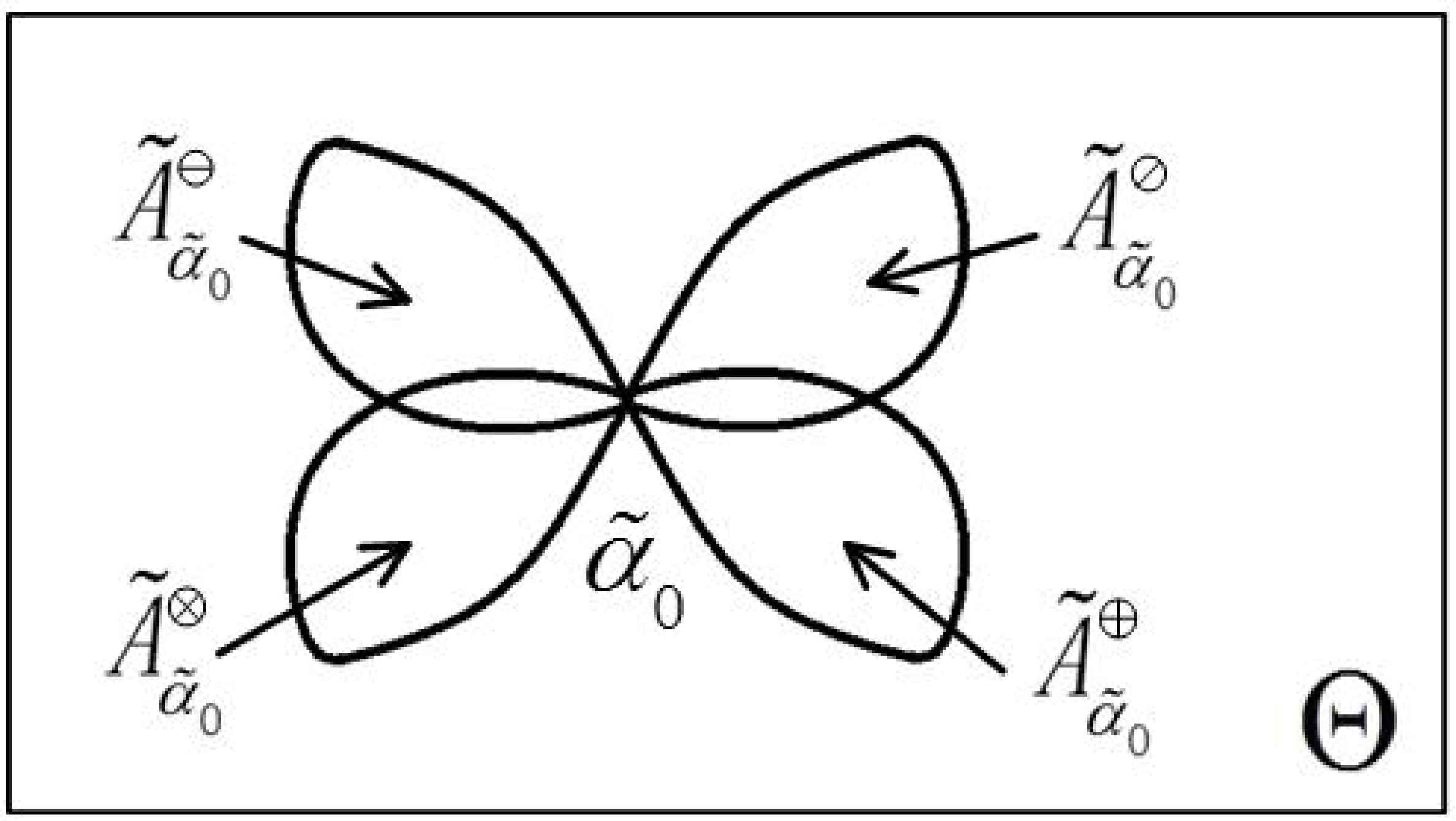
The relations of these four sets A˜α˜0⊕ , A˜α˜0⊝ , A˜α˜0⊗ , and A˜α˜0⊘ derived from ᾶ0 and the set of all the IVIFVs Θ can be shown by the following figure:

Firgue 1.

The relations of the addition, subtraction, multiplication and division regions
Based on the above results, we give the following definition:

Definition 10.

Assume that ᾶ1, ᾶ2,ᾶ3 and ᾶ4 are four IVIFVs. If α˜1∈A˜α˜0⊕ , α˜2∈A˜α˜0⊝ , α˜3∈A˜α˜0⊗ , and α˜4∈A˜α˜0⊘ , then ᾶ1 is called an addition change value for ᾶ0, ᾶ2 a subtraction change value for ᾶ0, ᾶ3 a multiplication change value for ᾶ0, and ᾶ4 a division change value for ᾶ0, respectively.

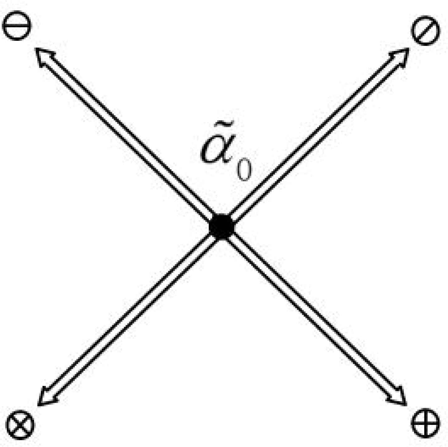
If α˜1∈A˜α˜0⊕ , α˜2∈A˜α˜0⊝ , α˜3∈A˜α˜0⊗ and α˜4∈A˜α˜0⊘ , then there must exist the IVIFVs β˜1 , β˜2 , β˜3 and β˜4 , such that α˜1=α˜0⊕β˜1 , α˜2=α˜0⊝β˜2 , α˜3=α˜0⊗β˜3 , and α˜4=α˜0⊘β˜4 . Therefore, an IVIFV has four change directions which can be shown visually by Figure 2. This is quite different from a real number which has only two change directions.

Figure 2.

The four different change directions

4. The sequences of IVIFVs

4.1. Various sequences of IVIFVs

Definition 11.

Suppose that {ᾶn} (n = 1,2,···) are a sequence of IVIFVs, that is to say, every ᾶn is an IVIFV in the sequence. If ∃N ∈ N+, and ∀n > N, α˜n∈A˜α˜0⊕ , where “∃” means “there exists” and “∀” means “for any”, then such {ᾶn} is called an addition sequence derived from ᾶ0 ; If ∀n > N, α˜n∈A˜α˜0⊝ , then {ᾶn} is a subtraction sequence derived from ᾶ0.

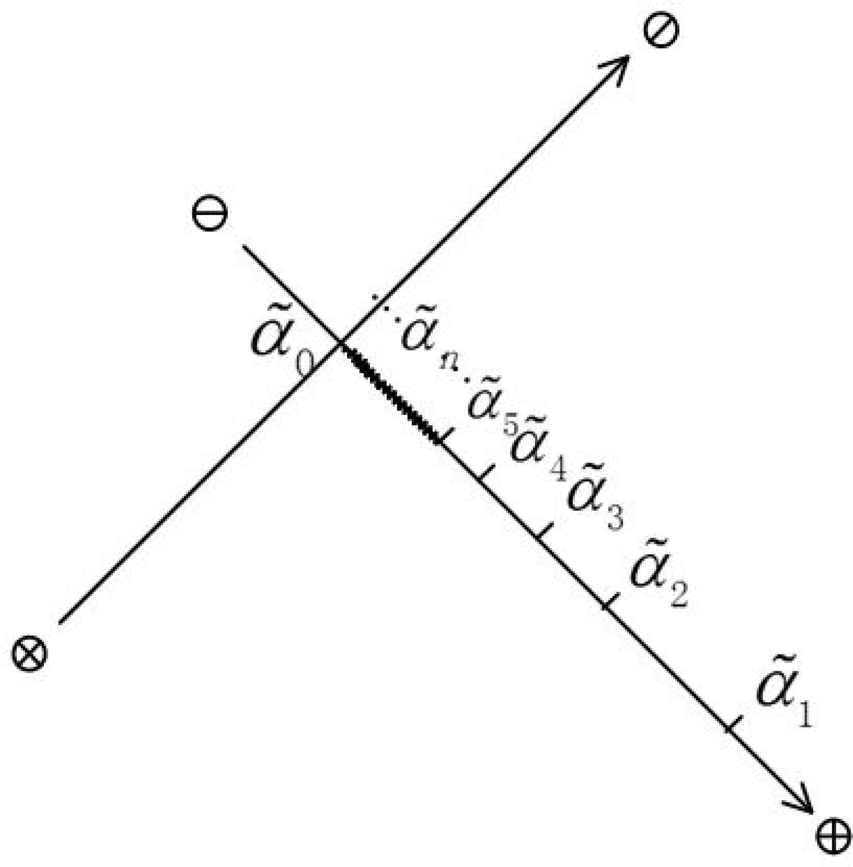
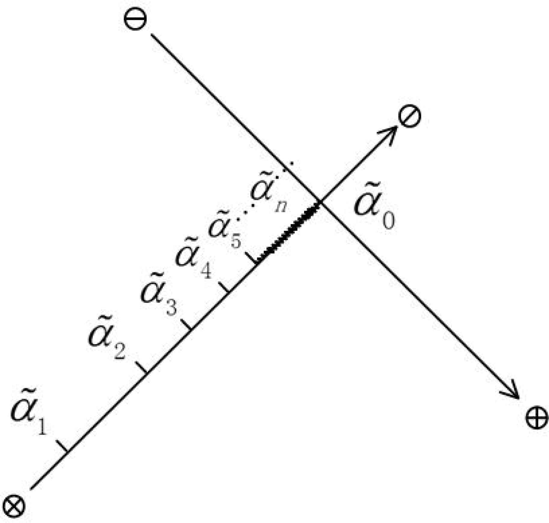
According to the above concepts, for a fixed IVIFV ᾶ0, we can always find the unlimited elements of an addition sequence derived from ᾶ0, which are all contained in A˜α˜0⊕ (see Figure 3); and the unlimited elements of a subtraction sequence of ᾶ0 completely contained in A˜α˜0⊝ (see Figure 4):

Figure 3.

An addition sequence of ᾶ0

Figure 4.

A subtraction sequence of ᾶ0

Definition 12.

Assume that {ᾶn} (n = 1,2,···) are a sequence of IVIFVs. If ∃N ∈ N+, ∀n > N, α˜n∈A˜α˜0⊘ , then we call {ᾶn} a division sequence derived from ᾶ0 ; If ∀n > N, α˜n∈A˜α˜0⊗ , then we call {ᾶn} a multiplication sequence derived from ᾶ0.

Similarly, from Figure 5, we can see that there are unlimited elements of a division sequence derived from ᾶ0 which are all in the set A˜α˜0⊘ . At the same time, from Figure 6, we can see the unlimited elements of a multiplication sequence derived from ᾶ0 which are all in A˜α˜0⊗ :

Figure 5.

A division sequence of ᾶ0

Figure 6.

A multiplication sequence of ᾶ0

4.2. The limits of various sequences of IVIFVs

In real number field, we use the distance | b − a | of two real numbers a and b to describe their approaching degree. The smaller the distance | b − a | is, the closer the two numbers are. a is infinitely approaching b if and only if the distance | b − a | is infinitely approaching to zero. How to describe the approaching process of two IVIFVs by using their basic operations? For arbitrary IVIFV ᾶ, because α˜⊕([0,0],[1,1])=α˜,α˜⊕θ˜→α˜ if only both the membership degree interval and the non-membership degree interval of θ˜ approach to those of the IVIFV ([0,0],[1,1]) . Therefore, we define the following limit process ᾶn → ᾶ0 :

Definition 13.

For an addition sequence derived from ᾶ0, denoted by {ᾶn} (n = 1,2,⋯), if ∀ε˜=([aε˜,bε˜],[cε˜,dε˜])>L([0,0],[1,1]) , ∃N ∈ N+, when ∀n > N, we have

α˜n⊝α˜0<Lε˜

Then we call ᾶ0 the addition limit of {ᾶn} as n → +∞, denoted by limn→+∞α˜n=α˜0⊕ or α˜n→α˜0⊕ .

Definition 13 shows that when ᾶn ⊝ ᾶ0 → ([0,0],[1,1]), we have α˜n→α˜0⊕ . Similarly, we give the following definition if each element ᾶn of a sequence is contained in A˜α˜⊝ :

Definition 14.

Let {ᾶn} be a subtraction sequence derived from ᾶ0. If ∀ε˜=([aε˜,bε˜],[cε˜,dε˜])>L([0,0],[1,1]) , ∃N ∈ N+,, when ∀n > N, we have

α˜0⊝α˜n<Lε˜
then ᾶ0 is called the subtraction limit of {ᾶn} as n → +∞, denoted by limn→+∞α˜n=α˜0⊝ or α˜n→α˜0⊝ .

We have considered the situations α˜n∈A˜α˜0⊕ and α˜n∈A˜α˜0⊝ , and defined the addition and subtraction limits respectively. Next we shall consider the situations when α˜n∈A˜α˜0⊗ and α˜n∈A˜α˜0⊘ . Because α˜⊗([1,1],[0,0])=α˜,α˜⊗θ˜→α˜ so long as both the membership degree interval and the non-membership degree interval of θ˜ approach to those of ([1,1],[0,0]), in the following, we shall give the other two limit definitions:

Definition 15.

Suppose that {ᾶn} is a division sequence derived from ᾶ0 . If ∀ε˜=([aε˜,bε˜],[cε˜,dε˜])<L([1,1],[0,0]) , ∃N ∈ N+, when ∀n > N, we have

α˜0⊘α˜n>Lε˜
then ᾶ0 is the division limit of {ᾶn} as n → +∞, denoted by limn→+∞α˜n=α˜0⊘ or α˜n→α˜0⊘ .

Definition 15 shows that when ᾶ0 ⊘ ᾶn → ([1,1],[0,0]), we have α˜n→α˜0⊘ .

Definition 16.

Assume that {ᾶn} is a multiplication sequence derived from ᾶ0 . If ∀ε˜=([aε˜,bε˜],[cε˜,dε˜])<L([1,1],[0,0]) , ∃N ∈ N+, when ∀n > N, we have

α˜n⊘α˜0>Lε˜
then ᾶ0 is the multiplication limit of {ᾶn} as n → +∞, denoted by limn→+∞α˜n=α˜0⊗ or α˜n→α˜0⊗ .

Next, we shall give an equivalent characterization of Definition 13. We first make an analysis on Definition 13. Because {ᾶn} is an addition sequence derived from ᾶ0, we can get

α˜n⊝α˜0=([an−a01−a0,bn−b01−b0],[cnc0,dnd0])∈Θ

Then Definition 13 shows that for any given aε˜>0 , bε˜>0 , cε˜<1 , dε˜<1 , we have an−a01−a0<aε˜ , bn−b01−b0<bε˜ and cnc0>cε˜ , dnd0>dε˜ . Thus by Definition 13, we know an − a0 → 0, bn − b0 → 0 and cnc0→1 , dnd0→1 simultaneously. Therefore, we can get the following equivalent characterization of Definition 13:

Theorem 1.

Let {ᾶn} be an addition sequence derived from ᾶ0, with ᾶn = ([an,bn],[cn,dn]) and ᾶ0 = ([a0,b0],[c0,d0]), then limn→+∞α˜n=α˜0⊕ if and only if limn→+∞an=a0 , limn→+∞bn=b0 and limn→+∞cn=c0 , limn→+∞dn=d0 .

Proof (Sufficiency).

Suppose that limn→+∞an=a0 , limn→+∞bn=b0 and limn→+∞cn=c0 , limn→+∞dn=d0 . By the definition of limit in real number field:

  1. (1)

    ∀ε1 > 0, ∃N1 ∈ N+, when ∀n > N1, we have

    an−a0<(1−a0)ε1

  2. (2)

    ∀ε2 > 0, ∃N2 ∈ N+, when ∀n > N2, we have

    bn−b0<(1−b0)ε2

  3. (3)

    ∀ε3 > 0, ∃N3 ∈ N+, when ∀n > N3, we have

    1−cnc0<ε3⇒cnc0>1−ε3

Similarly, ∀ε4 > 0, ∃N4 ∈ N+, when ∀n > N4, we have

1−dnd0<ε4⇒dnd0>1−ε4

Let N = max(N1,N2,N3,N4), then when ∀n > N, we have an−a01−a0<ε1 , bn−b01−b0<ε2 and cnc0>1−ε3 , dnd0>1−ε4 . In this case, if we take ε˜=([ε1,ε2],[1−ε3,1−ε4]) , then limn→+∞α˜n=α˜0⊕ .

(Necessity). If limn→+∞α˜n=α˜0⊕ , by Definition 13, ∀ε˜=([aε˜,bε˜],[cε˜,dε˜])>L([0,0],[1,1]) , ∃N ∈ N+, when ∀n > N, we have

α˜n⊝α˜0<Lε˜

That is,

([an−a01−a0,bn−b01−b0],[cnc0,dnd0])<L([aε˜,bε˜],[cε˜,dε˜])

As {ᾶn} is an addition sequence derived from ᾶ0, then 0<an−a01−a0<aε˜ , 0<bn−b01−b0<bε˜ and 1>cnc0>cε˜ , 1>dnd0>dε˜ . By the squeeze theorem of limit in real number field, we can get limn→+∞an=a0 , limn→+∞bn=b0 and limn→+∞cn=c0 , limn→+∞dn=d0 . Thus we complete the proof of Theorem 1.

Furthermore, when {ᾶn} is a subtraction sequence, a division sequence or a multiplication sequence derived from ᾶ0, we have the similar conclusion.

5. The continuity and differentiability of IVIFFs

5.1. The concept and properties of IVIFFs

Suppose that ᾶ = ([a,b],[c,d]), and F is a function of IVIFVs, that is,

F(α˜)=([f1(a,b,c,d),f2(a,b,c,d)],[g1(a,b,c,d),g2(a,b,c,d)])

If 0 ≤ fi(a,b,c,d) ≤ 1, 0 ≤ gi(a,b,c,d) ≤ 1, i = 1,2, and 0 ≤ f2 (a,b,c,d) + g2(a,b,c,d) ≤ 1, then we call the function F(ᾶ) an interval-valued intuitionistic fuzzy function (IVIFF) of ᾶ .

For brevity, we denote any given IVIFF

F(α˜)=([f1(a,b,c,d),f2(a,b,c,d)],      [g1(a,b,c,d),g2(a,b,c,d)])
as F = ([f1, f2],[g1, g2]).

Because F(ᾶ) ⊝ (ᾶ0) isn’t always an IVIFV, for the purpose of discussing the derivatives of IVIFFs, we want to know in what conditions F(ᾶ) ⊝ F(ᾶ0) will be an IVIFV. This question relates to the subtraction operation of IVIFV:

Definition 17.

Let F(α˜)=([f1(a,b,c,d),f2(a,b,c,d)],      [g1(a,b,c,d),g2(a,b,c,d)]) be an IVIFF of ᾶ = ([a,b],[c,d]), then we denote

S˜⊕(α˜0,F)={α˜|α˜∈A˜α˜0⊕,0≤g1(a,b,c,d)g1(a0,b0,c0,d0)≤1−f1(a,b,c,d)1−f1(a0,b0,c0,d0)≤1,                        0≤g2(a,b,c,d)g2(a0,b0,c0,d0)≤1−f2(a,b,c,d)1−f2(a0,b0,c0,d0)≤1}
as the addition area of F(ᾶ) at ᾶ0.

Using the subtraction operation of IVIFV, we can get

F(α˜)⊝F(α˜0)=([f1(a,b,c,d),f2(a,b,c,d)],[g1(a,b,c,d),g2(a,b,c,d)])⊝([f1(a0,b0,c0,d0),f2(a0,b0,c0,d0)],[g1(a0,b0,c0,d0),g2(a0,b0,c0,d0)])=([f1(a,b,c,d)−f1(a0,b0,c0,d0)1−f1(a0,b0,c0,d0),f2(a,b,c,d)−f2(a0,b0,c0,d0)1−f2(a0,b0,c0,d0)],       [g1(a,b,c,d)g1(a0,b0,c0,d0),g2(a,b,c,d)g2(a0,b0,c0,d0)])

From the analysis above, we know that ∀α˜∈S˜⊕(α˜0,F) , F(ᾶ) ⊝ F(ᾶ0) is still an IVIFV when ᾶ ⊝ ᾶ0 is an IVIFV.

Definition 18.

Suppose that F(α˜)=([f1(a,b,c,d),f2(a,b,c,d)],      [g1(a,b,c,d),g2(a,b,c,d)]) is an IVIFF of ᾶ = ([a,b],[c,d]), then we denote

S˜⊝(α˜0,F)={α˜|α˜∈A˜α˜0⊝,0≤g1(a0,b0,c0,d0)g1(a,b,c,d)≤1−f1(a0,b0,c0,d0)1−f1(a,b,c,d)≤1,                                    0≤g2(a0,b0,c0,d0)g2(a,b,c,d)≤1−f2(a0,b0,c0,d0)1−f2(a,b,c,d)≤1}
as the subtraction area of F(ᾶ) at ᾶ0.

By Definition 18, we know that ∀α˜∈S˜⊝(α˜0,F) , F(ᾶ0) ⊝ F(ᾶ) is still an IVIFV when ᾶ0 ⊝ ᾶ is an IVIFV.

Like the addition and subtraction areas of F(ᾶ) at ᾶ0, we can define the corresponding division and multiplication areas:

Definition 19.

Assume that F(α˜)=([f1(a,b,c,d),f2(a,b,c,d)],      [g1(a,b,c,d),g2(a,b,c,d)]) is an IVIFF of ᾶ = ([a,b],[c,d]), then we denote

S˜⊘(α˜0,F)={α˜|α˜∈A˜α˜0⊘,0≤f1(a0,b0,c0,d0)f1(a,b,c,d)≤1−g1(a0,b0,c0,d0)1−g1(a,b,c,d)≤1,                        0≤f2(a0,b0,c0,d0)f2(a,b,c,d)≤1−g2(a0,b0,c0,d0)1−g2(a,b,c,d)≤1}
as the division area of F(ᾶ) at ᾶ0.

Definition 20.

For an IVIFF F(α˜)=([f1(a,b,c,d),f2(a,b,c,d)],      [g1(a,b,c,d),g2(a,b,c,d)]) of ᾶ, we denote

S˜⊗(α˜0,F)={α˜|α˜∈A˜α˜0⊗,0≤f1(a,b,c,d)f1(a0,b0,c0,d0)≤1−g1(a,b,c,d)1−g1(a0,b0,c0,d0)≤1,                        0≤f2(a,b,c,d)f2(a0,b0,c0,d0)≤1−g2(a,b,c,d)1−g2(a0,b0,c0,d0)≤1}
as the multiplication area of F(ᾶ) at ᾶ0.

From Definitions 19 and 20, we know that ∀α˜∈S˜⊘(α˜0,F) , F(ᾶ0) ⊘ F(ᾶ) is still an IFV when ᾶ0 ⊝ ᾶ is an IVIFV, and ∀α˜∈S˜⊗(α˜0,F) , F(ᾶ0) ⊘ F(ᾶ) is still an IVIFV when ᾶ0 ⊝ ᾶ is an IVIFV.

In the following, we shall investigate the relationships of the previous results by some simple examples:

  1. (1)

    If F(ᾶ) = ᾶ, then f1(a,b,c,d) = a, f2(a,b,c,d) = b and g1(a,b,c,d) = c, g2(a,b,c,d) = d . If ∀α˜∈A˜α˜0⊕ , then we can get 0≤cc0≤1−a1−a0≤1 and 0≤dd0≤1−b1−b0≤1 . So ∀α˜∈A˜α˜0⊕ , we have

    0≤g1(a,b,c,d)g1(a0,b0,c0,d0)≤1−f1(a,b,c,d)1−f1(a0,b0,c0,d0)≤1
    and
    0≤g2(a,b,c,d)g2(a0,b0,c0,d0)≤1−f2(a,b,c,d)1−f2(a0,b0,c0,d0)≤1
    that is, S˜⊕(α˜0,F)=A˜α˜0⊕ . Similarly, we can also get
    S˜⊝(α˜0,F)=A˜α˜0⊝, S˜⊘(α˜0,F)=A˜α˜0⊘, S˜⊗(α˜0,F)=A˜α˜0⊗

  2. (2)

    If

    F(X˜)=X˜⊕α˜1=([a+a1−aa1,b+b1−bb1],[cc1,dd1])
    where X˜=([a,b],[c,d]) and ᾶ1 = ([a1,b1],[c1,d1]) .

    Let

    f1(a,b,c,d)=a+a1−aa1f2(a,b,c,d)=b+b1−bb1
    and
    g1(a,b,c,d)=cc1,g2(a,b,c,d)=dd1

    For any α˜∈A˜α˜0⊕ , we have 0≤cc0≤1−a1−a0≤1 and 0≤dd0≤1−b1−b0≤1 , which are equivalent to

    0≤cc1c0c1≤1−(a+a1−aa1)1−(a0+a1−a0a1)≤1
    and
    0≤dd1d0d1≤1−(b+b1−bb1)1−(b0+b1−b0b1)≤1
    respectively, which means that the following inequalities hold:
    0≤g1(a,b,c,d)g1(a0,b0,c0,d0)≤1−f1(a,b,c,d)1−f1(a0,b0,c0,d0)≤10≤g2(a,b,c,d)g2(a0,b0,c0,d0)≤1−f2(a,b,c,d)1−f2(a0,b0,c0,d0)≤1

    Therefore, S˜⊕(α˜0,F)=A˜α˜0⊕ . Similarly, we have S˜⊝(α˜0,F)=A˜α˜0⊝ .

  3. (3)

    For the case that

    IIFWAw(α˜1,α˜2,…α˜n)=([1−∏j=1n(1−aj)wj,1−∏j=1n(1−bj)wj], [∏j=1ncjwj,∏j=1ndjwj])
    where ᾶj = ([aj,bj],[cj,dj]), j = 1,2,…,n . For ∀α˜j′∈A˜α˜j⊕ , with α˜j′=([aj′,bj′],[cj′,dj′]) , we can get
    cj′cj≤(1−aj′)(1−aj)⇔(cj′cj)wj≤(1−aj′1−aj)wj⇔(cj′)wj∏i=1i≠jnciwicjwj∏i=1i≠jnciwi≤(1−aj′)wj∏i=1i≠jn(1−ai)wi(1−aj)wj∏i=1i≠jn(1−ai)wi
    and
    dj′dj≤(1−bj′)(1−bj)⇔(dj′dj)wj≤(1−bj′1−bj)wj⇔(dj′)wj∏i=1i≠jndiwidjwj∏i=1i≠jndiwi≤(1−bj′)wj∏i=1i≠jn(1−bi)wi(1−bj)wj∏i=1i≠jn(1−bi)wi

    Then we get S˜⊕(α˜j,IIFWA)=A˜α˜j⊕ . Similarly, we have S˜⊝(α˜j,IIFWA)=A˜α˜j⊝ .

  4. (4)

    For the case that

    IIFWGw(α˜1,α˜2,…α˜n)=([∏j=1najwj,∏j=1nbjwj],[1−∏j=1n(1−cj)wj,1−∏j=1n(1−dj)wj])
    where ᾶj = ([aj,bj],[cj,dj]), j = 1,2,…,n . For ∀α˜j′∈A˜α˜j⊘ , with α˜j′=([aj′,bj′],[cj′,dj′]) , it follows that
    ajaj′≤1−cj1−cj′⇔(ajaj′)wj≤(1−cj1−cj′)wj⇔(aj)wj∏i=1i≠jnaiwi(aj′)wj∏i=1i≠jnaiwi≤(1−cj)wj∏i=1i≠jn(1−ci)wi(1−cj′)wj∏i=1i≠jn(1−ci)wi
    and
    bjbj′≤1−dj1−dj′⇔(bjbj′)wj≤(1−dj1−dj′)wj⇔(bj)wj∏i=1i≠jnbiwi(bj′)wj∏i=1i≠jnbiwi≤(1−dj)wj∏i=1i≠jn(1−di)wi(1−dj′)wj∏i=1i≠jn(1−di)wi
    then S˜⊘(α˜j,IIFWG)=A˜α˜j⊘ . We can also obtain S˜⊗(α˜j,IIFWG)=A˜α˜j⊗ in a similar way.

5.2. The continuity of IVIFF

In real number field, the continuity of a real function f(x) is a very important property. If f(x) − f(x0) → 0 when x → x0, then the function f(x) is continuous. After defining the convergence of sequences of IVIFVs, it is natural for us to ask what the continuity of an IVIFF is. In the following, we shall focus on this issue:

Definition 21.

Let F(X˜) be an IVIFF of X˜ . If ∀ε˜=([aε˜,bε˜],[cε˜,dε˜])>L([0,0],[1,1]) , ∃δ˜=([aδ,bδ],[cδ,dδ]) , for any X˜∈S˜⊕(X˜0,F) , when ([0,0],[1,1])<LX˜⊝X˜0<Lδ˜ , there is F(X˜)⊝F(X˜0)<Lε˜ , then F(X˜) is continuous at X˜0 in the addition area, denoted by limX˜→X˜0⊕F(X˜)=F(X˜0) .

Definition 21 shows that if F(X˜) is continuous at X˜0 in the addition area S˜⊕(X˜0,F) , then when X˜⊝X˜0→([0,0],[1,1]) , we have F(X˜)⊝F(X˜0)→([0,0],[1,1]) .

Definition 22.

Suppose that F(X˜) is an IVIFF of X˜ . If ∀ε˜=([aε˜,bε˜],[cε˜,dε˜])>L([0,0],[1,1]) , ∃δ˜=([aδ,bδ],[cδ,dδ]) , making ∀X˜∈S˜⊝(X˜0,F) and ([0,0],[1,1])<LX˜0⊝X˜<Lδ˜ , such that F(X˜0)⊝F(X˜)<Lε˜ . Then F(X˜) is continuous at X˜0 in the subtraction area, denoted by limX˜→X˜0⊝F(X˜)=F(X˜0) .

Definition 23.

Assume that F(X˜) is an IVIFF of X˜ . If ∀ε˜=([aε˜,bε˜],[cε˜,dε˜])<L([1,1],[0,0]) , ∃δ˜=([aδ,bδ],[cδ,dδ]) , such that X˜∈S˜⊘(X˜0,F) and δ˜<LX˜0⊘X˜<L([1,1],[0,0]) satisfy F(X˜0)⊘F(X˜)>Lε˜ , then F(X˜) is continuous at X˜0 in the division area, denoted by limX˜→X˜0⊘F(X˜)=F(X˜0) .

Definition 24.

For a given IVIFF F(X˜) of X˜ , if ∀ε˜=([aε˜,bε˜],[cε˜,dε˜])<L([1,1],[0,0]) , ∃δ˜=([aδ,bδ],[cδ,dδ]) , for arbitrary X˜∈S˜⊗(X˜0,F) when δ˜<LX˜⊘X˜0<L([1,1],[0,0]) , the inequality F(X˜)⊘F(X˜0)>Lε˜ holds, then F(X˜) is continuous at X˜0 in the multiplication area, denoted by limX˜→X˜0⊗F(X˜)=F(X˜0) .

5.3. The differentiability of IVIFFs

As we all know, in the real number field, the derivativeness of a real function f(x) at a real number x depends on the existence of the following limit:

limx′→xf(x′)−f(x)x′−x

If f(x′) − f(x) ↛ 0, then the above limit might be equal to the worthless infinity. But, if f(x) is continuous, then limx′→xf(x′)−f(x)x′−x might be equal to a constant, and then we can gain the derivative of the function f(x) at a real number x:

df(x)dx=limx′→xf(x′)−f(x)x′−x.

Under interval-valued intuitionistic fuzzy environment, we try to use the idea of gaining the derivative of a real function to define the derivative of an IVIFF. We first analyze the value of limα˜′→α˜⊕F(α˜′)⊝F(α˜)α˜′⊝α˜ . From Definition 13, we know that ᾶ′ ⊝ ᾶ → ([0,0],[1,1]) when ᾶ′ → ᾶ⊕ . Then based on the subtraction operation of IVIFVs introduced in Section 2, on the one hand, if F(ᾶ′) ⊝ F(ᾶ) ↛ ([0,0],[1,1]), then the value limα˜′→α˜⊕F(α˜′)⊝F(α˜)α˜′⊝α˜ is equal to the IVIFV ([0,0],[1,1]) that takes no information about the divisor and the dividend, and is given only for satisfying the closure of division. On the other hand, so long as the function F(ᾶ) is continuous, the value F(ᾶ′) ⊝ F(ᾶ) will approach ([0,0],[1,1]) when ᾶ′ ⊝ ᾶ → ([0,0],[1,1]). So in this case we can catch the value limα˜′→α˜⊕F(α˜′)⊝F(α˜)α˜′⊝α˜ , which would not always equal to the IVIFV ([0,0],[1,1]).

After the above analysis, we first give the derivative of an IVIFF at an IVIFV ᾶ in the addition direction:

Definition 25.

If limα˜′→α˜⊕F(α˜′)⊝F(α˜)α˜′⊝α˜ is an IVIFV, then the function F(ᾶ) is called to be differentiable at ᾶ in the addition direction, and the limit value is called the derivative of F(ᾶ) at ᾶ.

Then we give the following necessary and sufficient condition for the differentiability of an IVIFF F(ᾶ):

Theorem 2.

Let F(α˜)=([f1(a,b,c,d),f2(a,b,c,d)],                  [g1(a,b,c,d),g2(a,b,c,d)]) be an IVIFF of ᾶ = ([a,b],[c,d]), then F(ᾶ) is differentiable in the addition direction of ᾶ, if and only if

{∂f1(a,b,c,d)∂b=∂f1(a,b,c,d)∂c=∂f1(a,b,c,d)∂d=0∂f2(a,b,c,d)∂a=∂f2(a,b,c,d)∂c=∂f2(a,b,c,d)∂d=0∂g1(a,b,c,d)∂a=∂g1(a,b,c,d)∂b=∂g1(a,b,c,d)∂d=0∂g2(a,b,c,d)∂a=∂g2(a,b,c,d)∂b=∂g2(a,b,c,d)∂c=0
and
{0≤1−a1−f1(a,b,c,d)∂f1(a,b,c,d)∂a≤10≤cg1(a,b,c,d)∂g1(a,b,c,d)∂c≤10≤1−b1−f2(a,b,c,d)∂f2(a,b,c,d)∂b≤dg2(a,b,c,d)∂g2(a,b,c,d)∂d≤1

Under the above sufficient and necessary condition, and F(ᾶ) = ([f1(a), f2(b)],[g1(c), g2(d)]), the derivative F(ᾶ) at ᾶ can be calculated as follows:

dF(α˜)dα˜=([1−a1−f1(a)f1′ (a),1−b1−f2(b)f2′ (b)],                      [1−cg1(c)g1′(c),1−dg2(d)g2′(d)])

Proof.

Let

α˜′=([a+Δa,b+Δb],[c+Δc,d+Δd])=           ([a′,b′],[c′,d′])∈S˜⊕(α˜,F)
then
F(α˜′)=([f1(a′,b′,c′,d′),f2(a′,b′,c′,d′)],                   [g1(a′,b′,c′,d′),g2(a′,b′,c′,d′)])

For brevity, we use the following notations in the proof process:

(I′)=(a′,b′,c′,d′), (I)=(a,b,c,d)

Thus,

dF(α˜)dα˜=limα˜′→α˜⊕F(α˜′)⊝F(α˜)α˜′⊝α˜=lima′→ab′→bc′→cd′→d([f1(I′),f2(I′)],[g1(I′),g2(I′)])⊝([f1(I),f2(I)],[g1(I),g2(I)])([a′,b′],[c′,d′])⊝([a,b],[c,d])=lima′→ab′→bc′→cd′→d([f1(I′)−f1(I)1−f1(I),f2(I′)−f2(I)1−f2(I)],[g1(I′)g1(I),g2(I′)g2(I)])([a′−a1−a,b′−b1−b],[c′c,d′d])=lima′→ab′→bc′→cd′→d([f1(I′)−f1(I)1−f1(I)1−aa′−a,f2(I′)−f2(I)1−f2(I)1−bb′−b],                [g1(I′)g1(I)−c′c1−c′c,g2(I′)g2(I)−d′d1−d′d])=([lima′→ab′→bc′→cd′→df1(I′)−f1(I)1−f1(I)1−aa′−a,lima′→ab′→bc′→cd′→df2(I′)−f2(I)1−f2(I)1−bb′−b],           [lima′→ab′→bc′→cd′→dg1(I′)g1(I)−c′c1−c′c,lima′→ab′→bc′→cd′→dg2(I′)g2(I)−d′d1−d′d])

We first consider the left endpoint of the membership degree interval:

lima′→ab′→bc′→cd′→df1(I′)−f1(I)1−f1(I)1−aa′−a=lima′→ab′→bc′→cd′→d1−a1−f1(I)f1(I′)−f1(I)a′−a=lima′→ab′→bc′→cd′→d1−a1−f1(I)[f1(a′,b′,c′,d′)a′−a−f1(a,b′,c′,d′)a′−a+           (f1(a,b′,c′,d′)b′−b−f1(a,b,c′,d′)b′−b)b′−ba′−a+           (f1(a,b,c′,d′)c′−c−f1(a,b,c,d′)c′−c)c′−ca′−a+           (f1(a,b,c,d′)d′−d−f1(a,b,c,d)d′−d)d′−da′−a]=1−a1−f1(I)(∂f1(I)∂a+∂f1(I)∂blima′→ab′→bc′→cd′→db′−ba′−a+     ∂f1(I)∂clima′→ab′→bc′→cd′→dc′−ca′−a+∂f1(I)∂dlima′→ab′→bc′→cd′→dd′−da′−a)

Similarly, we can get the right endpoint of the membership degree interval:

lima′→ab′→bc′→cd′→df2(I′)−f2(I)1−f2(I)1−bb′−b=lima′→ab′→bc′→cd′→d1−b1−f2(I)f2(I′)−f2(I)b′−b=1−b1−f2(I)(∂f2(I)∂b+∂f2(I)∂alima′→ab′→bc′→cd′→da′−ab′−b+      ∂f2(I)∂clima′→ab′→bc′→cd′→dc′−cb′−b+∂f2(I)∂dlima′→ab′→bc′→cd′→dd′−db′−b)

Next we calculate the part of the non-membership interval. We first consider the left endpoint of the non-membership degree interval:

lima′→ab′→bc′→cd′→dg1(I′)g1(I)−c′c1−c′c=lima′→ab′→bc′→cd′→d[cg1(I)×g1(I′)c−c′−c′c−c′]=lima′→ab′→bc′→cd′→d{cg1(I)[g1(a′,b′,c′,d′)−g1(a′,b′,c,d′)c−c′+g1(a′,b′,c,d′)−g1(a,b′,c,d′)a−a′a−a′c−c′+g1(a,b′,c,d′)−g1(a,b,c,d′)b−b′b−b′c−c′+g1(a,b,c,d′)−g1(a,b,c,d)d−d′d−d′c−c′+g1(a,b,c,d)c−c′]−c′c−c′}=1−cg1(I)[∂g1(I)∂c+∂g1(I)∂alima′→ab′→bc′→cd′→da′−ac′−c+∂g1(I)∂blima′→ab′→bc′→cd′→db′−bc′−c+∂g1(I)∂dlima′→ab′→bc′→cd′→dd′−dc′−c]

Likewise, we get the right endpoint of the non-membership degree interval as follows:

lima′→ab′→bc′→cd′→dg2(I′)g2(I)−d′d1−d′d=lima′→ab′→bc′→cd′→d[dg2(I)×g2(I′)d−d′−d′d−d′]=1−dg2(I)[∂g2(I)∂d+∂g2(I)∂alima′→ab′→bc′→cd′→da′−ad′−d+∂g2(I)∂blima′→ab′→bc′→cd′→db′−bd′−d+∂g2(I)∂clima′→ab′→bc′→cd′→dc′−cd′−d]

To ensure the derivative to be only the IVIFV, which doesn’t change with ᾶ, we have

{∂f1(a,b,c,d)∂b=∂f1(a,b,c,d)∂c=∂f1(a,b,c,d)∂d=0∂f2(a,b,c,d)∂a=∂f2(a,b,c,d)∂c=∂f2(a,b,c,d)∂d=0∂g1(a,b,c,d)∂a=∂g1(a,b,c,d)∂b=∂g1(a,b,c,d)∂d=0∂g2(a,b,c,d)∂a=∂g2(a,b,c,d)∂b=∂g2(a,b,c,d)∂c=0
and
{0≤1−a1−f1(a,b,c,d)∂f1(a,b,c,d)∂a≤10≤cg1(a,b,c,d)∂g1(a,b,c,d)∂c≤10≤1−b1−f2(a,b,c,d)∂f2(a,b,c,d)∂b≤dg2(a,b,c,d)∂g2(a,b,c,d)∂d≤1

Thus F(ᾶ) = ([f1(a), f2(b)],[g1(c), g2(d)]), and then

dF(α˜)dα˜=([1−a1−f1(a)f1′ (a),1−b1−f2(b)f2′ (b)],                     [1−cg1(c)g1′(c),1−dg2(d)g2′(d)])
which completes the proof.

In a similar way, we can get the derivative of F(ᾶ) at ᾶ in the subtraction direction. When α˜′∈S˜⊝(α˜,F) , we have

dF(α˜)dα˜=limα˜′→α˜⊝F(α˜)⊝F(α˜′)α˜⊝α˜′=([1−a1−f1(a)f1′ (a),1−b1−f2(b)f2′ (b)],[1−cg1(c)g1′(c),1−dg2(d)g2′(d)])

If the value dF(α˜)dα˜ is an IVIFV, then we call it the derivative of F(ᾶ) at ᾶ in the subtraction direction.

We find that the derivative values of F(ᾶ) at ᾶ in the addition and subtraction directions are exactly the same if f1, f2 and g1, g2 are derivable. So we shall unify the two kinds of derivatives into one.

Definition 26.

If the IVIFF F(ᾶ) is differentiable at ᾶ in its addition and subtraction directions, then we call

dF(α˜)dα˜=([1−a1−f1(a)f1′ (a),1−b1−f2(b)f2′ (b)],                     [1−cg1(c)g1′(c),1−dg2(d)g2′(d)])
the subtraction derivative of F(ᾶ) at ᾶ .

Theorem 2 gives a condition for the existence of an IVIFF’s subtraction derivative. This is just like the “C-R condition” in the complex number field.

In what follows, we shall study the subtraction derivatives of some special IVIFFs:

  1. (1)

    If F(X˜)=α˜0=([a0,b0],[c0,d0]) , then

    f1(a)=a0,f2(b)=b0,g1(c)=c0,g2(d)=d0,dF(X˜)dX˜=([0,0],[1,1])

  2. (2)

    If F(X˜)=X˜⊕α˜0=([a+a0−aa0,b+b0−bb0],[cc0,dd0]) , then

    f1(a)=a+a0−aa0,f2(b)=b+b0−bb0,g1(c)=cc0,g2(d)=dd0dF(X˜)dX˜=([1−a1−a−a0+aa0(1−a0),1−b1−b−b0+bb0(1−b0)],[1−ccc0c0,1−ddd0d0])=([1,1],[0,0])

  3. (3)

    If F(X˜)=α˜0⊗X˜=([a0a,b0b],[c0+c−c0c,d0+d−d0d]) , then

                   f1(a)=a0a,f2(b)=b0b,g1(c)=c0+c−c0c,g2(d)=d0+d−d0ddF(X˜)dX˜=([1−a1−a0aa0,1−b1−b0bb0],[1−cc0+c−c0c(1−c0),1−dd0+d−d0d(1−d0)])=([a0−a0a1−a0a,b0−b0b1−b0b],[c0c0+c−c0c,d0d0+d−d0d])=([a0,b0],[c0,d0])⊗([1−a1−a0a,1−b1−b0b],[1−cc0+c−c0c,1−dd0+d−d0d])
    1. (a)

      When ᾶ0 = ([a0,b0],[c0,d0]) = ([1,1],[0,0]), we get

      dF(X˜)dX˜=([1−a1−a,1−b1−b],[0,0])=([1,1],[0,0])

    2. (b)

      When ᾶ0 = ([a0,b0],[c0,d0]) = ([0,0],[1,1]), we have

      dF(X˜)dX˜=([0,0],[1c0+c−c0c,1d0+d−d0d])               =([0,0],[1,1])

      Because

      a0−a0a1−a0a=a01−a1−a0a≤a0,b0−b0b1−b0b=b01−b1−b0b≤b0
      and
      c0c+c0−c0c=c01c+c0(1−c)≥c0,d0d+d0−d0d=d01d+d0(1−d)≥d0

      Then we can get

      ([a0−a0a1−a0a,b0−b0b1−b0b],[c0c0+c−c0c,d0d0+d−d0d])≤L([a0,b0],[c0,d0])

  4. (4)

    If F(X˜)=λ·X˜=([1−(1−a)λ,1−(1−b)λ],[cλ,dλ]),0<λ≤1 , then

    f1(a)=1−(1−a)λ, f2(b)=1−(1−b)λ, g1(c)=cλ, g2(d)=dλdF(X˜)dX˜=([1−a(1−a)λλ(1−a)λ−1,1−b(1−b)λλ(1−b)λ−1],[1−λ,1−λ])                =([λ,λ],[1−λ,1−λ])

    The examples (5) and (6) below show that in interval-valued intuitionistic fuzzy environment, for any two functions F(X˜)=KX˜+α˜ and G(X˜)=KX˜+β˜ whether K is an IVIFV or a positive real number, we have dF(X˜)dX˜=dG(X˜)dX˜ . This conclusion is similar to the one in the real number field.

  5. (5)

    If G(X˜)=α˜⊗X˜⊕β˜ , then

    α˜⊗X˜⊕β˜=([aαa+aβ−aαaβa,bαb+bβ−bαbβb],                 [cβc+cαcβ−cαcβc,dβd+dαdβ−dαdβd])f1(a)=aαa+aβ−aαaβa,   f2(b)=bαb+bβ−bαbβbg1(c)=cβc+cαcβ−cαcβc,  g2(d)=dβd+dαdβ−dαdβddG(X)dX=([1−a1−(aαa+aβ−aαaβa)(aα−aαaβ),                   1−b1−(bαb+bβ−bαbβb)(bα−bαbβ)],                   [1−ccβc+cαcβ−cαcβc(cβ−cαcβ),                   1−ddβd+dαdβ−dαdβd(dβ−dαdβ)])=([aα−aαa1−aαa,bα−bαb1−bαb],[cαcα+c−cαc,dαdα+d−dαd])

    Let F(X˜)=α˜⊗X˜ , then we get dG(X˜)dX˜=dF(X˜)dX˜ .

  6. (6)

    If G(X˜)=λX˜⊕β˜ , λ > 0, then

    λX˜⊕β˜=([1−(1−a)λ+aβ(1−a)λ,1−(1−b)λ+bβ(1−b)λ],[cλcβ,dλdβ])f1(a)=1−(1−a)λ+aβ(1−a)λ, f2(b)=1−(1−b)λ+bβ(1−b)λg1(c)=cλcβ, g2(d)=dλdβdG(X˜)dX˜=([λ,λ],[1−λ,1−λ])

    Let F(X˜)=λX˜ , then we get dG(X˜)dX˜=dF(X˜)dX˜ .

    At last, as a special IVIFF, we examine the derivative of the IIFWA operator:

  7. (7)

    If

    IIFWAω(α˜1,α˜2,…,α˜n)=([1−∏j=1n(1−aj)ωj,1−∏j=1n(1−bj)ωj],[∏j=1ncjωj,∏j=1ndjωj])
    then
    f1(aj)=1−∏j=1n(1−aj)ωj,  f2(bj)=1−∏j=1n(1−bj)ωj;g1(cj)=∏j=1ncjωj,  g2(dj)=∏j=1ndjωj
    where ᾶj = ([aj,bj], [cj,dj]), and then
    d(IIFWAω(α˜1,α˜2,⋯,α˜n))dα˜i=([1−aj∏j=1n(1−aj)ωjωi∏j=1j≠in(1−aj)ωj(1−aj)ωi−1,1−bj∏j=1n(1−bj)ωjωi∏j=1j≠in(1−bj)ωj(1−bj)ωi−1],[1−cj∏j=1ncjωjωi∏j=1j≠incjωj·cjωi−1,1−dj∏j=1ndjωjωi∏j=1j≠indjωj·djωi−1])=([ωi,ωi],[1−ωi,1−ωi])

    As defined before, the change value for an IVIFV has four different change directions: the addition, subtraction, multiplication and division directions. We have discussed the addition and subtraction derivatives for an IVIFF. In the following, we shall consider the differentiability of an IVIFF in the multiplication and division directions:

Definition 27.

If limα˜′→α˜⊘(F(α˜)F(α˜′)⊝α˜α˜′) is an IVIFV, then we call F(ᾶ) to be differentiable at ᾶ in the division direction, and the limit value is called the derivative of F(ᾶ) at ᾶ .

Theorem 3.

Suppose that F(ᾶ) = ([f1(a,b,c,d), f2(a,b,c,d)],[g1(a,b,c,d), g2(a,b,c,d)]) is an IVIFF of ᾶ = ([a,b],[c,d]), then F(ᾶ) is differentiable at ᾶ in the division direction if and only if

{∂f1(a,b,c,d)∂b=∂f1(a,b,c,d)∂c=∂f1(a,b,c,d)∂d=0∂f2(a,b,c,d)∂a=∂f2(a,b,c,d)∂c=∂f2(a,b,c,d)∂d=0∂g1(a,b,c,d)∂a=∂g1(a,b,c,d)∂b=∂g1(a,b,c,d)∂d=0∂g2(a,b,c,d)∂a=∂g2(a,b,c,d)∂b=∂g2(a,b,c,d)∂c=0
and
{0≤af1(a,b,c,d)∂f1(a,b,c,d)∂a≤10≤1−c1−g1(a,b,c,d)∂g1(a,b,c,d)∂c≤10≤1−d1−g2(a,b,c,d)∂g2(a,b,c,d)∂d≤bf2(a,b,c,d)∂f2(a,b,c,d)∂b≤1

Under such sufficient and necessary condition, F(ᾶ) can be expressed by F(ᾶ) = ([f1(a), f2(b)],[g1(c), g2(d)]), and then the derivative F(ᾶ) at ᾶ in the division direction can be computed as:

lF(α˜)lα˜=([1−af1(a)f1′(a),1−bf2(b)f2′(b)], 1−c1−g1(c)g1′(c),1−d1−g2(d)g2′(d)])

When α′∈S˜⊗(α,F) , similarly, we have

lF(α˜)lα˜=limα˜′→α˜⊗(F(α˜′)F(α˜)⊝α˜′α˜)   =([1−af1(a)f1′(a),1−bf2(b)f2′(b)],         [1−c1−g1(c)g1′(c),1−d1−g2(d)g2′(d)])

If the limit value is an IVIFV, then we call it the derivative of F(ᾶ) at ᾶ in the multiplication direction.

As we can see, there are exactly the same derivative values in the division and multiplication directions if the functions f1, f2 and g1, g2 are derivable. So we also unify the two derivatives into one:

Definition 28.

If the IVIFF F(ᾶ) is differentiable at ᾶ in the division and multiplication directions, then

lF(α˜)lα˜=([1−af1(a)f1′(a),1−bf2(b)f2′(b)], [1−c1−g1(c)g1′(c),1−d1−g2(d)g2′(d)])
is called the division derivative of F(ᾶ) at ᾶ .

In the following, let’s see the division derivatives of some special IVIFFs:

  1. (1)

    If F(X˜)=α˜0=([a0,b0],[c0,d0]) , then

    f1(a)=a0,f2(b)=b0,g1(c)=c0,g2(d)=d0,lF(X˜)lX˜=([1,1],[0,0])

  2. (2)

    If F(X˜)=α˜0⊕X˜,              =([a0+a−a0a,b0+b−b0b],[c0c,d0d]) then

           f1(a)=a0+a−a0a,f2(b)=b0+b−b0b,      g1(c)=c0c,g2(d)=d0d   lF(X˜)lX˜=([1−aa0+a−a0a(1−a0),   1−bb0+b−b0b(1−b0)],[1−c1−c0cc0,1−d1−d0dd0])=([a0a0+a−a0a,b0b0+b−b0b],[c0−c0c1−c0c,d0−d0d1−d0d])=([a0,b0],[c0,d0])⊕([1−aa0+a−a0a,1−bb0+b−b0b],[1−c1−c0c,1−d1−d0d])≥L([a0,b0],[c0,d0])

  3. (3)

    If F(X˜)=α˜0⊗X˜=([a0a,b0b],[c0+c−c0c,d0+d−d0d]) , then

    f1(a)=a0a,f2(b)=b0b,g1(c)=c0+c−c0c,g2(d)=d0+d−d0dlF(X)lX=([1−aa0aa0,1−bb0bb0],     [1−c1−c−c0+c0c(1−c0),1−d1−d−d0+d0d(1−d0)])   =([0,0],[1,1])

  4. (4)

    If F(X˜)=X˜λ=([aλ,bλ],  [1−(1−c)λ,1−(1−d)λ]),0<λ≤1, , then

    f1(a)=aλ,f2(b)=bλ,g1(c)=1−(1−c)λ,g2(d)=1−(1−d)λlF(X˜)lX˜=([1−λ,1−λ],[1−c(1−c)λλ(1−c)λ−1,1−d(1−d)λλ(1−d)λ−1])=([1−λ,1−λ],[λ,λ])

  5. (5)

    If

    IIFWGω(α˜1,α˜2,…,α˜n)=  ([∏j=1najωj,∏j=1nbjωj],[1−∏j=1n(1−cj)ωj,1−∏j=1n(1−dj)ωj])
    then
    f1(a)=∏j=1najωj,f2(b)=∏j=1nbjωj,g1(c)=1−∏j=1n(1−cj)ωj,g2(d)=1−∏j=1n(1−dj)ωjl(IIFWGω(α˜1,α˜2,⋯,α˜n))lα˜i=([1−ai∏j=1najωjωi∏j=1j≠inajωj·aiωi−1,1−bi∏j=1nbjωjωi∏j=1j≠inbjωj·biωi−1],[1−ci∏j=1n(1−cj)ωjωi∏j=1j≠in(1−cj)ωj(1−ci)ωi−1,1−di∏j=1n(1−dj)ωjωi∏j=1j≠in(1−dj)ωj(1−di)ωi−1])=([1−ωi,1−ωi],[ωi,ωi])

6. The differentials of IVIFFs and their applications in approximate calculation

In real-life applications, we often encounter some complicated functions. If we compute the function value with the function itself, we shall need great effort. In some cases, we only need the approximate function value instead of the precise value. Using the differential, we can do it. In the following, we shall discuss the approximate calculation methods under interval-valued intuitionistic fuzzy environment.

To begin with, we give the concept of differential for IVIFFs. In the last section, we have defined two kinds of derivatives (the subtraction derivative and the division derivative), so we shall define two differential operations accordingly:

Definition 29.

For a given IVIFV ᾶ = ([a,b],[c,d]), we call A(ᾶ) = a and B(ᾶ) = b the take-value functions of membership interval and CL(ᾶ) = c, DR(ᾶ) = d the take-value functions of non-membership interval.

In what follows, we give the first kind of differential-the subtraction differential:

Definition 30.

Assume that Ỹ = F(ᾶ) = ([f1(a), f2(b)],[g1(c), g2(d)]) is an IVIFF and Δᾶ = ᾶ′ ⊝ ᾶ, then the concrete form of the subtraction differential of F(ᾶ) is defined as dF(α˜)dα˜⊗Δα˜ , denoted by dỸ, that is,

dY˜=dF(α˜)dα˜⊗Δα˜

The subtraction differential of the independent variable ᾶ is equal to Δᾶ . In fact,

dα˜=dF(α˜)=dF(α˜)dα˜⊗Δα˜=([1,1],[0,0])⊗Δα˜=Δα˜

So the subtraction differential of arbitrary IVIFF F(ᾶ) can be rewritten as:

dY˜=dF(α˜)dα˜⊗dα˜

Theorem 4.

Let Ỹ = F(ᾶ) = ([f1(a), f2(b)],[g1(c), g2(d)]) be an IVIFF, if F(ᾶ) has the subtraction derivative at ᾶ, and α˜′∈S˜⊕(α˜,F) , then we have

F(α˜′)⊝F(α˜)≈dF(α˜)dα˜⊗(α˜′⊝α˜)
that is ΔỸ ≈ dỸ, which satisfies the following conditions:
limΔa→0A(ΔY˜)−A(dY˜)Δa=0,    lim Δb→0B(ΔY˜)−B(dY˜)Δb=0limΔc→0C(ΔY˜)−C(dY˜)Δc=0,    limΔd→0D(ΔY˜)−D(dY˜)Δd=0

Proof.

For any α˜∈S˜⊕(α˜,F) , we have

Δα˜=α˜′⊝α˜=([a′,b′],[c′,d′])⊝([a,b],[c,d])       =([a′−a1−a,b′−b1−b],[c′c,d′d])
and
dF(α˜)dα˜=([1−a1−f1(a)f1′(a),1−b1−f2(b)f2′(b)],[1−cg1(c)g1′(c),1−dg2(d)g2′(d)])

So we can get

dY˜=dF(α˜)dα˜⊗Δα˜=([a′−a1−f1(a)f1′(a),b′−b1−f2(b)f2′(b)], [1−c−c′g1(c)g1′(c),1−d−d′g2(d)g2′(d)])F(α˜)⊕(dF(α˜)dα˜⊗Δα˜)=([f1(a),f2(b)],[g1(c),g2(d)])⊕([a′−a1−f1(a)f1′(a),b′−b1−f2(b)f2′(b)],[1−c−c′g1(c)g1′(c),1−d−d′g2(d)g2′(d)])=([f1(a)+(a′−a)f1′(a),f2(b)+(b′−b)f2′(b)],      [g1(c)+(c′−c)g1′(c),g2(d)+(d′−d)g2′(d)])=([f1(a)+f1′(a)−f1(a)+o(a′−a),f2(b)+f2′(b)−f2(b)+o(b′−b)],[g1(c)+g1′(c)−g1(c)+o(c′−c),g2(d)+g2′(d)−g2(d)+o(d′−d)])=([f1′(a)+o(a′−a),f2′(b)+o(b′−b)],      [g1′(c)+o(c′−c),g2′(d)+o(d′−d)])≈F(α˜′)

Thus, we have F(α˜′)⊝F(α˜)≈dF(α˜)dα˜⊗(α˜′⊝α˜) , that is, ΔỸ ≈ dỸ, and

limΔa→0A(ΔY˜)−A(dY˜)Δa=0,    lim Δb→0B(ΔY˜)−B(dY˜)Δb=0limΔc→0C(ΔY˜)−C(dY˜)Δc=0,    limΔd→0D(ΔY˜)−D(dY˜)Δd=0

Similarly, we have

F(α˜)⊝F(α˜′)≈dF(α˜)dα˜⊗(α˜⊝α˜′)  when α˜′∈S˜⊝(α˜,F).

Below, we compute the approximate values of some IVIFFs to demonstrate the effectiveness of Theorem 4:

Example 1.

Let Ỹ = F(ᾶ) = λ · ᾶ,(0 < λ ≤ 1), so f1(a) = 1 − (1 − a)λ, f2(b) = 1 − (1 − b)λ and g1(c) = cλ, g2(d) = dλ. By the definition of derivative of IVIFF, we have

dF(α˜)dα˜=([λ,λ],[1−λ,1−λ])

Furthermore, by Theorem 4, we can get

F(α˜⊕Δα˜)⊝F(α˜)≈([λ,λ],[1−λ,1−λ])⊗Δα˜

On the other hand, by the operational laws of IVIFVs λ(ᾶ1 ⊕ ᾶ2) = λᾶ1 ⊕ λᾶ2, we have

F(α˜⊕Δα˜)⊝F(α˜)=λ(α˜⊕Δα˜)⊝λα˜=λΔα˜

Suppose that Δᾶ = ([0.01,0.02],[0.96,0.97]), and λ = 0.3, then

dY˜=([λ,λ],[1−λ,1−λ])⊗Δα˜=([0.003,0.006],[0.988,0.991])ΔY˜=λΔα˜=([0.0030,0.0060],[0.9878,0.9909])

From the above results, we can find that the value of dỸ is very close to the one of ΔỸ.

Next, we consider a common decision making problem:

Example 2.

Assume that three experts give their evaluation values using the IVIFVs: ᾶ1 = ([0.2,0.3],[0.3,0.4]), ᾶ2 = ([0.1,0.2],[0.2,0.5]) and ᾶ3 = ([0.1,0.2],[0.2,0.3]) for an alternative, and their weight vector is ω = (0.2,0.4,0.4)T . Using the IIFWA operator, we can calculate their overall value:

IIFWAω(α˜1,α˜2,α˜3)=([1−∏j=13(1−aj)ωj,1−∏j=13(1−bj)ωj],  [∏j=13cjωj,∏j=13djωj])=([1−(1−0.2)0.2×(1−0.1)0.4×(1−0.1)0.4,     [1−(1−0.3)0.2×(1−0.2)0.4×(1−0.2)0.4],      [0.30.2×0.20.4×0.20.4,0.40.2×0.50.4×0.30.4])=([0.121,0.221],[0.217,0.390])

But if some of the experts, for example, the first expert would like to adjust the value of ᾶ1 slightly and gives the new assessment α˜1′ , then we can deal with the information aggregation as follows:

If α˜1′∈S˜⊕(α˜1,F) , then there must exist an IVIFV β˜1 such that α˜1′=α˜1⊕β˜1 . Assume that α˜1′=([0.3,0.4],[0.2,0.3])∈S˜⊕(α˜1,F) , then β˜1=α˜1′⊝α˜1=([0.125,0.143],[0.667,0.75]) and

IIFWAω(α˜1′,α˜2,α˜3)≈IIFWAω(α˜1,α˜2,α˜3)⊕([ω1,ω1],[1−ω1,1−ω1])⊗(α˜1′⊝α˜1)=([0.121,0.221],[0.217,0.390])⊕([0.2,0.2],[0.8,0.8])⊗([0.125,0.143],[0.667,0.75])=([0.144,0.245],[0.2,0.368])

Based on the division derivative, we shall define the other kind of differential--the division differential:

Definition 31.

Suppose that Ỹ = F(ᾶ) = ([f1(a), f2(b)],[g1(c), g2(d)]) is an IVIFF and ∇α˜=α˜′⊘α˜=α˜′α˜ , then the division differential of F(ᾶ) is defined as lF(α˜)lα˜⊕∇α˜ , denoted by lỸ, that is,

lY˜=lF(α˜)lα˜⊕∇α˜

Similarly, for the identity function F(ᾶ) = ᾶ = ([a,b],[c,d]), when computing its division differential, we have lᾶ = ∇ᾶ, so the division differential can be rewritten as:

lY˜=lF(α˜)lα˜⊕lα˜

Theorem 5.

Let Ỹ = F(ᾶ) = ([f1(a), f2(b)],[g1(c), g2(d)]) be an IVIFF, if F(ᾶ) owns the division derivative at ᾶ, and α˜′∈S˜⊗(α˜,F) , then we get

F(α˜′)⊘F(α˜)≈lF(α˜)lα˜⊕(α˜′⊘α˜)

Noting that ∇Y˜=F(α˜′)⊘F(α˜)=F(α˜′)F(α˜) and ∇ᾶ = ᾶ′ ⊘ ᾶ, we have ∇Ỹ ≈ lỸ, satisfying the following conditions:

limΔa→0A(ΔY˜)−A(lY˜)Δa=0,    lim Δb→0B(ΔY˜)−B(lY˜)Δb=0limΔc→0C(ΔY˜)−C(lY˜)Δc=0,    limΔd→0D(ΔY˜)−D(lY˜)Δd=0

When α˜′∈S˜⊘(α˜,F) , we have

F(α˜)⊘F(α˜′)≈lF(α˜)lα˜⊕(α˜⊘α˜′)

Example 3.

If the IVIFF F(ᾶ) = ᾶλ,(0 < λ ≤ 1), that is, f1(a) = aλ, f2(b)= bλ, g1(a) = 1 − (1 − a)λ, g2(b) = 1 − (1 − b)λ, and

lF(X˜)lX˜=([1−λ,1−λ],[λ,λ])

By Theorem 5, we have

F(α˜⊗∇α˜)F(α˜)≈([1−λ,1−λ],[λ,λ])⊕∇α˜

Because (ᾶ1 ⊗ ᾶ2)λ = ᾶ1λ ⊗ ᾶ2λ, then we have

F(α˜⊗∇α˜)F(α˜)=(α˜⊗∇α˜)λα˜λ=(∇α˜)λ

If we suppose ∇ᾶ = ([0.90,0.92], [0.03,0.05]) and λ = 0.4, then we can get

([1−λ,1−λ],[λ,λ])⊕∇α˜=([0.96,0.968],[0.012,0.02])
and
(∇α˜)λ=([0.959,0.967],[0.012,0.020])
which shows that the approximate degree of replacing (∇ᾶ)λ with ([1 − λ, 1 − λ],[λ,λ]) ⊕ ∇ᾶ is very high.

From the proof process of Theorem 4, we can further derive the following conclusion:

Theorem 6.

Let Ỹ = F(ᾶ) = ([f1(a), f2(b)],[g1(c), g2(d)]) be an IVIFF which satisfies the conditions: f1″(a)=f2″(b)=g1″(c)=g2″(d)=0 and α˜′∈S˜⊕(α˜,F) , then

F(α˜′)⊝F(α˜)=dF(α˜)dα˜⊗(α˜′⊝α˜)

The same holds true for α˜′∈S˜⊝(α˜,F) , α˜′∈S˜⊗(α˜,F) or α˜′∈S˜⊘(α˜,F) .

Proposition 1 in Section 2 has shown several operation laws for IVIFVs, such as the commutative law and the distributive law between the scalar multiplication and addition operations. But the existence of the distributive laws between the multiplication and addition operations is still unknown. In the following, we shall discuss this question:

Example 4.

Assume ᾶ0 = ([a0,b0],[c0,d0]), ᾶ = ([a,b],[c,d]) and ᾶ′ = ([a′,b′],[c′,d′]) are three arbitrary IVIFVs, and let the IVIFF F(ᾶ) = ᾶ0 ⊗ ᾶ, in which f1(a) = a0a, f2(b) = b0b and g1 (c) = c0 + c − c0c, g2(d) = d0 + d − d0d . Obviously, f1″(a)=f2″(b)=g1″(c)=g2″(d)=0 . So by Theorem 6, we have

F(α˜⊕α˜′)⊝F(α˜)=dF(α˜)dα˜⊗α˜′

That is, F(α˜⊕α˜′)=F(α˜)⊕dF(α˜)dα˜⊗α˜′ .

By the example in Section 5, we can get

dF(α˜)dα˜=α˜0⊗([1−a1−a0a,1−b1−b0b],[1−cc0+c−c0c,1−dd0+d−d0d])

Then the following equation holds:

α˜0⊗(α˜⊕α˜′)=α˜0⊗α˜⊕α˜0⊗α˜′⊗([1−a1−a0a,1−b1−b0b],[1−cc0+c−c0c,1−dd0+d−d0d])

The above equation shows that ᾶ0 ⊗ (ᾶ ⊕ ᾶ′) ≠ ᾶ0 ⊗ ᾶ ⊕ ᾶ0 ⊗ ᾶ′, i.e., the distributive laws between the multiplication and addition operations is not correct.

7. Conclusions

In this paper, we have firstly presented the concepts of the change values of IVIFVs, based on which, we have classified the sequences of IVIFVs and given the limit definitions of these sequences respectively. Moreover, we have introduced the concept of IVIFF. After all these preparations, we have studied the continuities and derivatives (the subtraction and division derivatives) of IVIFFs. To make the concepts of derivatives of IVIFFs easier to be understood, we have illustrated them by some special IVIFFs. Based on the derivatives proposed previously, at the end of the paper, we have investigated two differential operations (the subtraction and division differentials) of IVIFFs and applied them in estimating the values of IVIFFs.

Acknowledgments

The work was supported by the National Natural Science Foundation of China (No.61273209) and the Central University Basic Scientific Research Business Expenses Project (No. skgt201501). The author also would like to thank the editor and the reviewers whose helpful comments have led to the improvements of the paper.

References

1.LA Zadeh, Fuzzy sets, Information and Control, Vol. 8, No. 3, 1965, pp. 338-353.
2.K Atanassov, Intuitionistic fuzzy sets, Fuzzy Sets and Systems, Vol. 20, No. 1, 1986, pp. 87-96.
3.E Szmidt and J Kacprzyk, Using intuitionistic fuzzy sets in group decision making, Control and Cybernetics, Vol. 31, No. 4, 2002, pp. 1037-1053.
4.ZS Xu, Intuitionistic fuzzy aggregation operators, IEEE Transactions on Fuzzy Systems, Vol. 15, No. 6, 2007, pp. 1179-1187.
5.ZS Xu, Intuitionistic preference relations and their application in group decision making, Information Sciences, Vol. 177, No. 11, 2007, pp. 2363-2379.
6.H Zhao, ZS Xu, SS Liu, and Z Wang, Intuitionistic fuzzy MST clustering algorithms, Computers & Industrial Engineering, Vol. 62, No. 4, 2012, pp. 1130-1140.
7.Z Wang, ZS Xu, SS Liu, and ZQ Yao, Direct clustering analysis based on intuitionistic fuzzy implication, Applied Soft Computing, Vol. 23, 2014, pp. 1-8.
8.HS Le and TT Nguyen, Intuitionistic fuzzy recommender systems: An effective tool for medical diagnosis, Knowledge-Based Systems, Vol. 74, 2015, pp. 133-150.
9.P Balasubramaniam and VP Ananthi, Image fusion using intuitionistic fuzzy sets, Information Fusion, Vol. 20, 2014, pp. 21-30.
10.CG Da Costa, B Bedregal, and ADD Neto, Atanassov’s intuitionistic fuzzy probability and Markov chains, Knowledge-Based Systems, Vol. 43, 2013, pp. 52-62.
11.MC Zheng, ZK Shi, and Y Liu, Triple I method of approximate reasoning on Atanassov’s intuitionistic fuzzy sets, International Journal of Approximate Reasoning, Vol. 55, No. 6, 2014, pp. 1369-1382.
12.B Dawaz, WA Dudek, and YB Jun, Intuitionistic fuzzy H-v-submodules, Information Sciences, Vol. 176, No. 3, 2006, pp. 285-300.
13.WJ Chen and SH Zhang, Intuitionistic fuzzy Lie sub-super algebras and intuitionistic fuzzy ideals, Computers and Mathematics with Applications, Vol. 58, No. 8, 2009, pp. 1645-1661.
14.Q Lei and Z Xu, Derivative and differential operations of intuitionistic fuzzy numbers, International Journal of Intelligent Systems, Vol. 30, No. 4, 2015, pp. 468-498.
15.Q Lei and ZS Xu, Fundamental properties of intuitionistic fuzzy calculus, Knowledge-Based Systems, Vol. 76, 2015, pp. 1-16.
16.Q Lei, ZS Xu, H Bustince, and J Fernandez, Intuitionistic fuzzy integrals based on Archimedean t-conorms and t-norms, Information Sciences, Vol. 327, 2016, pp. 57-70.
17.ZS Xu and RR Yager, Some geometric aggregation operators based on intuitionistic fuzzy sets, International Journal of General Systems, Vol. 35, No. 4, 2006, pp. 417-433.
18.XH Yu, ZS Xu, SS Liu, and Q Chen, On ranking of intuitionistic fuzzy values based on dominance relations, International Journal of Uncertainty, Fuzziness and Knowledge-Based Systems, Vol. 22, No. 2, 2014, pp. 315-335.
19.KH Guo, Amount of information and attitudinal-based method for ranking Atanassov’s intuitionistic fuzzy values, IEEE Tansactions on Fuzzy Systems, Vol. 22, No. 1, 2014, pp. 177-188.
20.XM Zhang and ZS Xu, A new method for ranking intuitionistic fuzzy values and its application in multi-attribute decision making, Fuzzy Optimization and Decision Making, Vol. 11, No. 2, 2012, pp. 135-146.
21.K Atanassov and G Gargov, Interval-valued intuitionistic fuzzy sets, Fuzzy Sets and Systems, Vol. 31, No. 3, 1989, pp. 343-349.
22.FF Jin, LD Pei, HY Chen, and LG Zhou, Interval-valued intuitionistic fuzzy continuous weighted entropy and its application to multi-criteria fuzzy group decision making, Knowledge-Based Systems, Vol. 59, 2014, pp. 132-141.
23.TY Chen, The extended linear assignment method for multiple criteria decision analysis based on interval-valued intuitionistic fuzzy sets, Applied Mathematical Modeling, Vol. 38, No. 7–8, 2014, pp. 2101-2117.
24.FY Meng, CQ Tan, and Q Zhang, The induced generalized interval-valued intuitionistic fuzzy hybrid Shapley averaging operator and its application in decision making, Knowledge-Based Systems, Vol. 42, No. 2, 2013, pp. 9-19.
25.H Zhao and ZS Xu, Group decision making with density-based aggregation operators under interval-valued intuitionistic fuzzy environments, Journal of Intelligent and Fuzzy Systems, Vol. 27, No. 2, 2014, pp. 1021-1033.
26.DF Li, Linear programming method for M ADM with interval-valued intuitionistic fuzzy sets, Expert Systems with Applications, Vol. 37, No. 8, 2010, pp. 5939-5945.
27.J Wu, HB Huang, and QW Cao, Research on AHP with interval-valued intuitionistic fuzzy sets and its application in multi-criteria decision making problems, Applied Mathematical Modelling, Vol. 37, No. 24, 2013, pp. 9898-9906.
28.ZS Xu, Methods for aggregating interval-valued intuitionistic fuzzy information and their application to decision making, Control and Decision, Vol. 22, No. 2, 2007, pp. 215-219.
29.J Wu and F Chiclana, A risk attitudinal ranking method for interval-valued intuitionistic fuzzy numbers based on novel attitudinal expected score and accuracy functions, Applied Soft Computing, Vol. 22, No. 5, 2014, pp. 272-286.
30.ZH Zhang, JY Yang, YP Ye, and QS Zhang, A generalized interval-valued intuitionistic fuzzy sets, Procedía Engineering, Vol. 15, 2011, pp. 2037-2041.
31.G Deschrijver and EE Kerre, On the relationship between some extensions of fuzzy set theory, Fuzzy Sets and Systems, Vol. 133, No. 2, 2003, pp. 227-235.
Journal
International Journal of Computational Intelligence Systems
Volume-Issue
9 - 1
Pages
36 - 56
Publication Date
2016/01/01
ISSN (Online)
1875-6883
ISSN (Print)
1875-6891
DOI
10.1080/18756891.2016.1144152How to use a DOI?
Copyright
© 2016. the authors. Co-published by Atlantis Press and Taylor & Francis
Open Access
This is an open access article under the CC BY-NC licence (http://creativecommons.org/licences/by-nc/4.0/).

Cite this article

TY  - JOUR
AU  - Hua Zhao
AU  - Zeshui Xu
AU  - Zeqing Yao
PY  - 2016
DA  - 2016/01/01
TI  - Interval-Valued Intuitionistic Fuzzy Derivative and Differential Operations
JO  - International Journal of Computational Intelligence Systems
SP  - 36
EP  - 56
VL  - 9
IS  - 1
SN  - 1875-6883
UR  - https://doi.org/10.1080/18756891.2016.1144152
DO  - 10.1080/18756891.2016.1144152
ID  - Zhao2016
ER  -