In this article we derive the triangular representations of the fundamental eigensolutions of the focusing 1 + 1 AKNS system with symmetric nonvanishing boundary conditions. Its continuous spectrum equals
∪[-iμ,iμ]
, where μ is the absolute value of the AKNS solution at spatial infinity. We also study the behavior of the scattering coefficients near the endpoints ±iμ of the branch cut, where we distinguish between the generic case and the exceptional case.
Nonlinear Schrödinger (NLS) equations have been fundamental in modeling nonlinear wave phenomena in plasmas [22,34], deep water surfaces [1,4,38], optical fibres [1,18,28], ferromagnetic materials [11,37], and Bose–Einstein condensates [26,27]. NLS equations with solutions decaying at infinity have been studied in detail [2–4,9,16]. After finding the Peregrine solutions [25], significant results on NLS equations with nonvanishing boundary conditions have been reported in Akhmediev et al. [5,6], Akhmediev and Korneev [7], Its et al. [19], Mihalache et al. [23], Tajiri and Watanabe [29], Zakharov and Gelash [35,36]. The direct and inverse scattering theory of the focusing NLS equation with nonvanishing boundary conditions has been studied systematically in Biondini and Kovačić [8], Demontis et al. [14]. We shall frequently refer to Demontis et al. [14] for some of the direct scattering results.
In this article we consider the focusing 1 + 1 AKNS system
vx=(-ikσ3+Q)v,(1.1)
where v is a function of
x∈
with values in
2
, σ3 = diag(1, −1), and
Q=(0q-q*0)
is the potential. We assume that there exist two distinct 2 × 2 matrices
Qr=(0qr-qr*0)
and
Ql=(0ql-ql*0)
satisfying μ = |qr| = |ql| > 0 such that for some s ≥ 0 the integrability condition
(Hs)∫0∞dy(1+|y|)s(∥Q(-y)-Ql∥+∥Q(y)-Qr∥)<+∞(1.2)
holds. Condition (1.2) is usually assumed for s = 0, 1. The Lax pair equations whose compatibility condition is equivalent to the focusing NLS equation, are discussed in detail in Appendix B (cf. [13]).
Under condition (H0) and for
k∈∪(-iμ,iμ)
, there exist two fundamental eigensolutionsΦ˜(x,k)
and
Ψ˜(x,k)
of (1.1) satisfying the asymptotic conditions
Φ˜(x,k)=exΛl(k)[I2+o(1)],x→-∞,(1.3a)
Ψ˜(x,k)=exΛr(k)[I2+o(1)],x→+∞,(1.3b)
where
Λl(k)=-ikσ3+Ql,Λr(k)=-ikσ3+Qr.(1.4)
Under condition (H1) the fundamental eigensolutions can be defined for
k∈∪[-iμ,iμ]
. Their existence can easily be proven by iterating the Volterra integral equations [14]
appears in (1.6) only as the argument of even functions and hence the sign indeterminacy in defining λ(k) by means of a square root does not affect (1.6).
In this article we derive in a rigorous way the triangular representations
Φ˜(x,k)=exΛl(k)+∫-∞xdyJ(x,y)eyΛl(k),(1.8a)
Ψ˜(x,k)=exΛr(k)+∫x∞dyK(x,y)eyΛr(k),(1.8b)
where for each
x∈
the integrability condition
∫-∞xdy∥J(x,y)∥+∫x∞dy∥K(x,y)∥<+∞(1.9)
holds. Triangular representations are well-known under vanishing boundary conditions [13,27–29] but have never been derived under integrability conditions of the form (1.9), with one notable exception. In Demontis et al. [14] the representations (1.8) have been derived under the conditions (H1) and
qx∈L1()
at the expense of replacing (1.9) by the quadratic integrability condition
∫-∞xdy∥J(x,y)∥2+∫x∞dy∥K(x,y)∥2<+∞.(1.10)
After establishing the triangular representations of the fundamental eigensolutions, we introduce the conformal mapping λ(k) by (1.7) and distinguish between left and right versions of k ∈(−iμ, iμ) as boundary points of the analytic manifolds
k∈𝕂±
in 1,1-correspondence with the complex half-planes
λ∈±
. We then go on to define the Jost functions and to derive their triangular representations. We also study in detail the conjugate transposition and conjugate non-transposition symmetries of the various quantities.
Once the triangular representations have been established, we go on studying the asymptotic behavior of the scattering coefficients as the spectral parameter k tends to ±iμ. In analogy with the case of the Schrödinger equation on the line [10,12,15], we shall make the distinction between the generic case where the corresponding Jost solutions are linearly independent, and the exceptional case where these solutions are proportional.
This paper is organized as follows. In Section 2 we establish the triangular representations of the fundamental eigensolutions. Their asymptotic behavior at either end of the real x-line will be the topic of Section 3. We then introduce the conformal mapping λ(k), define the Jost functions, and derive their triangular representations in Section 4. Section 5 is devoted to the conjugation symmetry properties of the various quantities. Next, in Section 6 we investigate the asymptotic behavior of the scattering coefficients near the endpoints of the branch cut k ∈[−iμ, iμ] and prove the integrability of the Fourier transforms of the reflection coefficients.
Finally, we discuss the contents of the various appendices. In Appendix A we discuss the Wiener algebra of constants plus Fourier transforms of L1-functions and invertibility within this algebra, well-known material treated at length in Gelfand et al. [17]. In this appendix we introduce the notation of writing Zn×m as the set of n × m matrices with entries in Z. The time dependence of the scattering data is discussed in Appendix B. To avoid clogging notations in the main body of the paper, we do not indicate any time dependence unless it is absolutely necessary.
2. TRIANGULAR REPRESENTATIONS
In this section we derive the triangular representations of the fundamental eigensolutions in a rigorous way. We also relate the potential to the integral kernels appearing in the triangular representations.
Factoring out the asymptotic behavior of the fundamental eigensolutions, we write
where the triangular representations (1.8) are putatively written as
M˜(x,k)=I2+∫0∞dαJ(x,x-α)e-αΛl(k),(2.4a)
N˜(x,k)=I2+∫0∞dαK(x,x+α)eαΛr(k).(2.4b)
We may thus convert the integral equations (2.3) into Volterra integral equations for the integral kernelsJ(x, x − α) and K(x, x + α). As in the vanishing case [3,13], we shall derive estimates for the integral kernels from the Volterra integral equations they satisfy.
Although at first sight the procedure explained in the past few lines may seem circular, below we shall in fact prove the existence of the integral kernels satisfying (1.9) by applying Gronwall’s inequality to the putative integral equations obtained by Fourier transforming the Volterra integral equations (2.3). By Fourier transformation of their unique solutions, we then arrive at the triangular representations for the fundamental eigensolutions satisfying (2.3), thus completing their proof.
The triangular representations (2.4) can be viewed as integral transforms of the type described by the following result.
Proposition 2.1.
Suppose the entries of F belong to
L1(+;(1+α)dα)
. Then the integral transform
Then (2.7) is true, while (2.8) implies
Fe(α)=F(α)±∫α∞dβF(β)Qr,l
and
Fo(β)=∫α∞dβF(β)σ3
. Consequently,
F(α)=Fe(α)±Fo(α)σ3Qr,l.(2.9)
We now observe that
F^(k)
does not change when changing the sign of λ while keeping k invariant. Decomposing
F^(k)
into k-even and k-odd functions of
k∈∪[-iμ,iμ]
, we obtain
We prove the triangular representation (2.11a) first, then use a symmetry argument to derive (2.11b) within a few lines, and then establish the second part of the theorem involving condition (Hs+1) for s = 0, 1, 2, … by going through the modifications required in the estimates. The second part for noninteger s ≥ 0 then follows by an interpolation argument.
We shall derive L1-estimates for the inhomogeneous term Finh(α) and the J-dependent term Fh(α) and then apply Gronwall’s inequality to obtain an L1-estimate for J.
Let us compute the inhomogeneous term on the right-hand side, splitting it into k-even and k-odd parts. Using
k2λ2=1-μ2λ2
, we get under condition (H2) for the k-even component of the inhomogeneous term
Applying (2.9) to compute the Fourier cosine transform of Finh(α), we see that the terms containing factors of the form
(sin(λα)λ)2
cancel out. Using (2.8) we get
Applying (2.9) to compute the Fourier cosine transform of Fh(α), we see that the terms containing factors of the form
(sin(λα)λ)2
cancel out. Unfortunately, only half the terms containing factors
sin(λα)λ
do. Using (2.8) we get
We now strip off the Fourier cosine transform using (2.8), directly in the terms containing a factor cos(λα) or
sin(λα)λ
and indirectly after interchanging α and β in the terms containing a factor cos(λβ) or
sin(λβ)λ
. To avoid repeating nearly similar estimates, we write the cosine transform terms as the Fourier cosine transforms of various matrix functions of the form
where z − α ≤ z and z − α ≤ 2x − z − α for each α ≥ 0. In fact,
𝒬=Q-Ql
and
𝒥=J
in the first three lines of (2.15),
𝒬=Ql[Q-Ql]
and
𝒥=J
in the fourth line of (2.15), and
𝒬=Q-Ql
and
𝒥=σ3Jσ3Ql
in the fifth line of (2.15). Integrating (2.16a) and (2.16b) with respect to
α∈+
we obtain the upper bounds
thus proving the triangular representation (2.11a).
The proof of the triangular representation (2.11b) is based on a simple parity symmetry argument. In fact, letting Q(#)(x) = Q(−x) we switch the roles of Qr and Ql by using
Qr,l(#)=Ql,r
and obtain the following symmetry relations for the fundamental eigensolutions:
Let us now prove the second part of the theorem for s = 0, 1, 2, …. Under the hypothesis (Hs+1), we modify the estimates (2.14), (2.17a), and (2.17b), where s = 0, 1, 2, …. Instead of (2.14) we get
Let us now derive expressions to pass from the (1, 2)-elements of the integral kernel J(x, y) and K(x, y) to the potential Q(x). These expressions have been derived by different means in Demontis et al. [14, Eq. (3.5)] under the assumption that (H2) is valid and
qx∈L1()
.
Theorem 2.2.
Under condition (H1) we have
J12(x,x)=12[q(x)-ql],K12(x,x)=-12[q(x)-qr].(2.21)
It suffices to extend the expression obtained in Demontis et al. [14] to general potentials satisfying (H1). Taking
α→0+
in the expression
Using (2.19) we see that, under condition (H1),
J(x,x)-12[Q(x)-Ql]
is a continuous function of
x∈
. Utilizing a continuity argument we easily extend (2.21) to arbitrary potentials satisfying (H1).
The proof for K(x, x) can in fact be obtained from the result for J(x, x) by using (2.20).
3. RELATING FUNDAMENTAL EIGENSOLUTIONS
To study the asymptotic behavior of the fundamental eigensolutions as x → ±∞, we write the Volterra integral equations (1.5) as follows [14, Eqs. (2.12)]:
is the evolution system associated with the first order system (1.1) associated with the piecewise constant potential Qf. Then [14, Eqs. (2.22) and (2.23)]
Φ˜(x,k)=Ψ˜(x,k)Bl(k),Ψ˜(x,k)=Φ˜(x,k)Br(k),(3.2)
where
Bl(k)=I2+∫-∞∞dy𝒢(0,y;k)[Q(y)-Qf(y)]Φ˜(y,k),(3.3a)
Br(k)=I2-∫-∞∞dy𝒢(0,y;k)[Q(y)-Qf(y)]Ψ˜(y,k),(3.3b)
are each other’s inverses.
Letting V(x, t) be a square matrix solution of the AKNS system (1.1), we easily derive for V−1 the “inverse” AKNS system
[V-1]x=-V-1VxV-1=-V-1(-ikσ3+Q)VV-1=V-1(ikσ3-Q).
Consequently, in analogy with (1.5) we obtain the Volterra integral equations
In this section we view (1.7) as a conformal mapping from a suitable k-manifold to a suitable λ-manifold and define the Jost functions. We also derive the triangular representations of the Jost functions. Finally, we introduce the scattering coefficients and the reflection coefficients and derive their representations as Fourier transforms.
4.1. Conformal Mapping
Let us now view
λ(k)=k2+μ2
as the conformal mapping from the complex k-plane
𝕂
cut along [−iμ, iμ] onto the complex λ plane
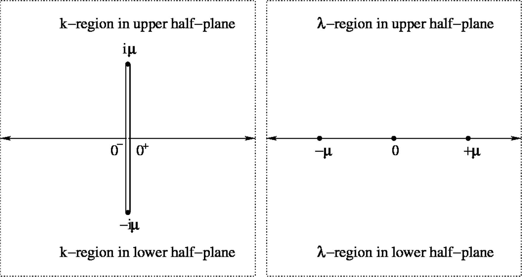
that satisfies λ ∼ k at infinity. Allowing each k ∈(−iμ, iμ) to have a left and a right copy to be put into 1, 1-correspondence with λ ∈(−μ, 0) and λ ∈(0, μ), respectively, we create diffeomorphisms between the analytic manifolds
𝕂±
and the open complex half-planes
±
and between the analytic manifolds with boundary
𝕂±∪∂𝕂±
and the closed complex half-planes
±∪
. Doing it this way, many functions can be interchangeably viewed as functions of k and as functions of λ (Figure 1).
Figure 1
The regions
k∈𝕂±
and
λ∈±
with manifold boundary. Note that
𝕂±
have the common boundary (−∞, −μ]∪[μ, +∞) and
±
have the real line as their common boundary.
The following Fourier representation is true [24, 10.22.61]:
is the Bessel function of order one. Obviously, the left-hand side of (4.1) is the Fourier transform of a function in
L1(+)
and hence is continuous in
λ∈+∪
, is analytic in
λ∈+
, and vanishes as λ → ∞ from within the closed upper half complex λ-plane. For
λ∈-∪
and
k∈𝕂-∪∂𝕂-
we obtain by complex conjugation
∫0∞dte-iλtJ1(μt)μt=∫-∞0dteiλtJ1(μt)μt=-iλ+k.(4.2)
4.2. Definition of Jost Functions
Letting
Wr,l(k)=(wr,l(1)(k)wr,l(2)(k))=I2-iλ+kσ3Qr,l
stand for the 2 × 2 matrix whose columns are the eigenvectors of Λr,l(k), i.e., letting
exΛr,l(k)Wr,l(k)=Wr,l(k)e-iλxσ3,(4.3)
we define the Jost functions as ϕ(x, k) and ψ(x, k) for
k∈𝕂+∪∂𝕂+
and
ψ¯(x,k)
and
ϕ¯(x,k)
for
k∈𝕂-∪∂𝕂-
as follows:
The Jost functions in (4.4a) can also be defined for
k∈𝕂-∪∂𝕂-
and those in (4.4b) for
k∈𝕂+∪∂𝕂+
by computing the corresponding columns of Wr,l(k) for k in the complementary manifold. For
0≠k∈
(and hence for λ ∈ (−∞, −μ] ∪ [μ, +∞) the Jost functions coincide when defined either way. For
k∈∂𝕂+∪∂𝕂-
we call
Φ(x,k)=(ϕ(x,k)ϕ¯(x,k)),Ψ(x,k)=(ψ¯(x,k)ψ(x,k)),
the Jost matrices.
4.3. Definition of Scattering Coefficients
Putting
S(k)=Wr(k)-1Bl(k)Wl(k),S¯(k)=Wl(k)-1Br(k)Wr(k),
where S(k) and
S¯(k)
are each other’s inverses, we obtain
and similarly for the entries of
S¯(k)
. Thus the scattering coefficients a(k) and c(k) are well-defined for
k∈𝕂+∪∂𝕂+
and for
k∈∂𝕂-
,
a¯(k)
and
c¯(k)
are well-defined for
k∈𝕂-∪∂𝕂-
and for
k∈∂𝕂+
, and the off-diagonal scattering coefficients for
k∈∪∂𝕂+∪∂𝕂-
, with the possible exception of k = ±iμ. The entries of s(k) and
S¯(k)
may not be defined for k = ±iμ but they are when multiplied by
2λλ+k
.
4.4. Triangular Representations of Jost Solutions
Using the triangular representations (2.11) and the Fourier representations (4.1) and (4.2), we get
Let us now apply the projections Π+ and Π− defined by (A.1) to (4.11). Applying the projections Π+ to (4.11a) and (4.11b) and Π− to (4.11c) and (4.11d), we obtain with the help of (A.1)
belong to
𝒲2×2
. The (1, 1)-element of (4.15a) and the (2, 2)-element of (4.15b) belong to
𝒲+
. The (2, 2)-element of (4.15a) and the (1, 1)-element of (4.15b) belong to
𝒲-
. Further,
2λλ+ka(k)-1
and
2λλ+kc(k)-1
belong to
𝒲+
,
2λλ+ka¯(k)-1
and
2λλ+kc¯(k)-1
to
𝒲-
, and
2λλ+kb(k)
,
2λλ+kb¯(k)
,
2λλ+kd(k)
, and
2λλ+kd¯(k)
to
𝒲
.
Using that
S(k)S¯(k)=I2=S¯(k)S(k)
, we obtain the identities
ρ(k)=-c(k)-1d¯(k),r(k)=-a(k)-1b¯(k),(4.17a)
ρ¯(k)=-c¯(k)-1d(k),r¯(k)=-a¯(k)-1b(k),(4.17b)
where for the moment we leave open the existence of the reciprocals in (4.16) and (4.17). Hence, proving the reflection coefficients to belong to
𝒲0
is postponed to Section 6.
5. SYMMETRIES
In this section we derive the matrix conjugate transpose symmetry properties and nontranspose conjugate symmetry properties for Jost functions and scattering and reflection coefficients. The dagger denotes the matrix conjugate transpose.
a. Conjugate transposition symmetry. For
k∈∪[-iμ,iμ]
the matrix functions
Ψ˜(x,k)-1
and
Ψ˜(x,k*)†
both satisfy the differential equation
Vx=V(x,t)(ikσ3-Q),
as do the matrix functions
Φ˜(x,k)-1
and
Φ˜(x,k*)†
. Thus,
Φ˜(x,k*)†=Φ˜(x,k)-1,Ψ˜(x,k*)†=Ψ˜(x,k)-1,(5.1)
where
k∈∪[-iμ,iμ]
. We observe that
k*=k
for
k∈
and
k*=-k
for k ∈[−iμ, iμ]. Thus for
k∈
the fundamental eigensolutions
Φ˜(x,k)
and
Ψ˜(x,k)
are unitary matrices of determinant 1. We also get
where in (5.4a) the choice of the sign in defining λ from k does not matter. In (5.4b) this choice is to be made consistently. Using (2.4), (3.8), and (5.4a) we obtain for the integral kernels
J(x,x-α)†=J˜(x-α,x),K(x,x+α)†=K˜(x+α,x),(5.5)
where
α∈+
.
Using (4.7) and (4.4) we obtain for the Jost matrices
Φ(x,k*)†=2λλ+kΦ(x,k)-1,(5.6a)
Ψ(x,k*)†=2λλ+kΨ(x,k)-1,(5.6b)
where
k∈𝕂+∪∂𝕂+
as far as the second row of (5.6a) and the first row of (5.6b) are concerned and
k∈𝕂-∪∂𝕂-
as far as the first row of (5.6b) and the second row of (5.6b) are concerned. Using (4.5) we obtain for the matrix of scattering coefficients
S(k*)†=S(k)-1=S¯(k),S¯(k*)†=S¯(k)=S(k).(5.7)
Thus S(k) and
S¯(k)
are unitary matrices if
k∈
. Since S(k) and
S¯(k)
both have unit determinant, we get
a(k*)*=a¯(k),c(k*)*=c¯(k),(5.8a)
b(k*)*=-b¯(k),d(k*)*=-d¯(k),(5.8b)
where
-iμ≠k∈𝕂-∪∂𝕂-
in (5.8a) and
-iμ≠k∈∂𝕂-
in (5.8b). Equations (4.16) imply that the reflection coefficients satisfy the symmetry relations
ρ¯(k)=-ρ(k*)*,r¯(k)=-r(k*)*,(5.9)
provided the reciprocals in their definitions (4.16) exist.
b. Conjugation symmetry. Let
σ2=(0-ii0)
stand for the second Pauli matrix. Then it is easily verified that
σ2Ψ˜(x,k*)*σ2
and
Ψ˜(x,k)
both satisfy the differential equation (1.1). The same thing is true for the other fundamental eigensolution
Φ˜
. We thus obtain
where in (5.14a) the choice of the sign in defining λ from k does not matter. In (5.14b) this choice is to be made consistently. Using (5.10) and (5.14b) we obtain for the Jost matrices
It is well-known that in the scattering theory of the Schrödinger equation on the line with Faddeev class potential two cases can be distinguished [10,12,15]: the generic case where for k = 0 the two Jost functions are linearly independent, and the exceptional case where for k = 0 the two Jost functions are linearly dependent. The scattering theory in the exceptional case is more easily developed by strengthening the integrability condition on the potential (as done in Chadan and Sabatier [10], Deift and Trubowitz [12] and Faddeev [15]), though such strengthening can be avoided at the expense of more complicated mathematical arguments [20]. For reflectionless potentials we are always in the exceptional case.
In the theory of the Schrödinger equation on the line with Faddeev class potential we can actually prove that there are no spectral singularities [12]. In fact, for positive energy k2 the two Jost functions can be proven to be linearly independent. In the present situation we actually need to assume absence of spectral singularities. Indeed, it is well-known that a(k) = c(k) for
0≠λ∈+∪
and
a¯(k)=c¯(k)
for
0≠λ∈-∪
. Therefore, throughout this article we assume absence of spectral singularities:
There do not exist any
0≠λ(k)∈
where a(k), c(k),
a¯(k)
, and
c¯(k)
vanish.
As a result, under this assumption the reflection coefficients ρ(k) and r(k) are well-defined for
iμ≠k∈𝕂+∪∂𝕂+
and the reflection coefficients
ρ¯(k)
and
r¯(k)
are well-defined for
-iμ≠k∈𝕂-∪∂𝕂-
. Moreover, b(k),
b¯(k)
, d(k), and
d¯(k)
are well-defined for
k∈∂𝕂+∪∂𝕂-
. Their definitions for k = ±iμ are a different matter to be pursued presently.
it is clear that the Jost functions ϕ(x, iμ) and ψ(x, iμ) are linearly independent iff the Jost functions
ψ¯(x,-iμ)
and
ϕ¯(x,-iμ)
are linearly independent. As in the Schrödinger case, we can therefore make a distinction between the following two cases:
(a)
the generic case: the Jost functions ϕ(x, iμ) and ψ(x, iμ) are linearly independent. OR: the Jost functions
ϕ¯(x,-iμ)
and
ψ¯(x,-iμ)
are linearly independent.
(b)
the exceptional case: the Jost functions ϕ(x, iμ) and ψ(x, iμ) are linearly dependent. OR: the Jost functions
ϕ¯(x,-iμ)
and
ψ¯(x,-iμ)
are linearly dependent.
Theorem 6.1.
Suppose condition (H1) is satisfied. Then we are in the generic case if and only if
limk→iμk∈𝕂+∪∂𝕂+2λλ+ka(k)
exists and is nonzero. If this limit vanishes, we are in the exceptional case.
Hence, in the exceptional case the (proportional) Jost functions ϕ(x, iμ) and ψ(x, iμ) are bounded in
x∈
and have finite nonzero limits as x → ± ∞.
Theorem 6.2.
Let us assume condition (H1) in the generic case and condition (H2) in the exceptional case, as well as absence of spectral singularities. Let us also assume that a(k) does not vanish as k → iμ. Then the reflection coefficients ρ(k),
ρ¯(k)
, r(k), and
r¯(k)
are Fourier transforms of functions in
L1()
. Moreover, there are only finitely many discrete eigenvalues.
In the absence of spectral singularities and in the generic case, the four reflection coefficients are all Fourier transforms of functions in
L1()
[cf. Appendix A]. Moreover, in this case there are at most finitely many discrete eigenvalues.
It remains to consider the exceptional case in detail. To do so, we strengthen the integrability assumption on the potential by assuming condition (H2). Since
2λλ+ka(k)
and
2λλ+kb(k)
can then easily be shown to be the Fourier transforms (in λ) of functions in
L1(+;(1+α)dα)
and
L1(;(1+|α|)dα)
, respectively, we can then apply Taylor’s theorem and write
a(k)=c(k)=a-1λ+a0+o(1),k→iμin𝕂+∪∂𝕂+,(6.2a)
b(k)=b-1λ+b0+o(1),k→iμin∂𝕂+,(6.2b)
where in the exceptional case we must have a−1 = 0. We need to prove that, in the exceptional case, a0 ≠ 0 and b−1 = 0. Equations (5.7) and (5.8) imply
where a(k) = c(k). Substituting (6.2) in the (2, 2)-element of either equation we get
b-1d-1=0,b-1d0+b0d-1=0,|a0|2+b0d0=|a0|2+b0*d0*=1.
Substituting (6.2) [with λ* = −λ] in the (1, 2)-element of the left equation we get
a0(d-1+b-1*)=0,a0d0=a0b0*.
The Ansatz b−1 = 0 and d−1 ≠ 0 leads to b0 = 0 and |a0| = 1, so that
d-1+b-1*=0
, a contradiction. In the same way we arrive at a contradiction from the Ansatz b−1 ≠ 0 and d−1 = 0. We must therefore conclude that b−1 = d–1 = 0. Instead of (6.2b), we thus arrive at the identities
b(k)=b0+o(1),d(k)=d0+o(1),(6.3)
where
b0d0=b0*d0*=1-|a0|2
is a real number. Furthermore,
This leads to two mutually exclusive possibilities:
(a)
a0≠0
,
d0=b0*
, and
|a0|2+|b0|2=|a0|2+|d0|2=1
.
(b)
a0 = 0 and b0d0 = 1. Since
a(k)[d(k)+b¯(k)]=0
with a(k) ≠ 0 for values of
k∈∂𝕂+
approaching iμ, the absence of spectral singularities assumption implies that |b0| = |d0|. Consequently, there exists a phase
θ∈
such that
b0=d0*=eiθ
.
In the former case the reflection coefficients are Fourier transforms of functions in
L1()
, whereas in the latter case the reflection coefficients blow up as k → iμ.
is well-defined. Thus the identity
ϕ=ψ¯a+ψb
implies that in the exceptional case
ϕ(x,iμ)=(b0-qr*μa0)ψ(x,iμ),
where the proportionality constant is nonzero. In the same way we prove that
ψ(x,iμ)=(d0-qlμa0)ϕ(x,iμ),
where the proportionality constant is nonzero as k = ±iμ. Since these two proportionality constants have product 1,
d0=b0*
, and
qlqr*=μ2ei(θl-θr)
, we get
(b0-e-iθra0)(b0*-eiθla0)=1.
The proof of Theorem 6.2 forced us to consider the mutually exclusive versions of the exceptional case, denoted by (a) and (b). In the generic case and in the exceptional case (a) the reflection coefficients are Fourier transforms of L1-functions. Unfortunately this is no longer the case in the exceptional case (b), the so-called hyperexceptional case for want of a better term. At present we cannot exclude the occurrence of the hyperexceptional case, but we are not aware of any focusing potential leading to the hyperexceptional case either.
CONFLICTS OF INTEREST
The author declares no conflicts of interest.
ACKNOWLEDGMENTS
The author is greatly indebted to Martin Klaus for discussions on 1 + 1 AKNS systems with nonvanishing boundary conditions and the occurrence of spectral singularities for piecewise constant potentials, and to Francesco Demontis for carefully reading the manuscript. The author has been partially supported by the Fondazione Banco di Sardegna in the framework of the research program Integro-Differential equations and non-local problems and by the Regione Autonoma della Sardegna in the framework of the research program Algorithms and models for imaging science, and by Istituto Nazionale della Alta Matematica, Gruppo Nazionale per la Fisica Matematica (INdAM-GNFM).
APPENDIX A
1. WIENER ALGEBRAS
By the (continuous) Wiener algebra
𝒲
we mean the complex vector space of constants plus Fourier transforms of L1-functions
𝒲={c+h^:c∈,h∈L1()}
endowed with the norm |c| + ||h||1. Here we define the Fourier transform as follows:
(h)(λ)=h^(λ)=∫-∞∞dyeiλyh(y)
. The invertible elements of the commutative Banach algebra
𝒲
with unit element are exactly those
c+h^∈𝒲
for which c ≠ 0 and
c+h^(λ)≠0
for each
λ∈
[17].
The algebra
𝒲
has the two closed subalgebras
𝒲+
and
𝒲-
consisting of those
c+h^
such that h is supported on
+
and
-
, respectively. The invertible elements of
𝒲±
are exactly those
c+h^∈𝒲±
for which c ≠ 0 and
c+h^(λ)≠0
for each
λ∈±∪
[17]. Letting
𝒲0±
and
𝒲0
stand for the (nonunital) closed subalgebras of
𝒲±
and
𝒲
consisting of those
c+h^
for which c = 0, we obtain the direct sum decomposition
𝒲=⊕𝒲0+⊕𝒲0-,𝒲0=𝒲0+⊕𝒲0-.
By Π± we now denote the (bounded) projection of
𝒲
onto
𝒲0±
along
⊕𝒲0∓
. Then Π+ and Π– are complementary projections. In fact,
(Π±f)(λ)=12πi∫-∞∞dζf(ζ)ζ-(λ±i0+),(A.1)
where
f∈𝒲0∩Lp()
for some p ∈ (1, +∞). These direct sum decompositions coupled by the Fourier transform can be schematically represented as follows:
L1()=L1(-)⊕L1(+)↓↓↓𝒲0=𝒲0-⊕𝒲0+
Now observe that
acts as an isometric linear 1, 1-correspondence from
L1()
onto
𝒲0
. If we define the norm of
⊕L1()
as
∥c+h∥=|c|+∥h∥1
, we obtain the direct sum decomposition
L1()=L1(+)⊕L1(-),
where the projection
-1Π±
is the restriction of an arbitrary
h∈L1()
to the half-line
±
.
Throughout this article we denote the vector spaces of n × m matrices with entries in
𝒲
,
𝒲±
, and
𝒲0±
by
𝒲n×m
,
𝒲±n×m
, and
𝒲0±n×m
, respectively. We write
L1()n×m
and
L1(±)n×m
for the vector spaces of n × m matrices with entries in
L1()
and
L1(±)
, respectively. Using a suitable (i.e., submultiplicative) matrix norm, we can turn all of these vector spaces into Banach spaces. It is then clear that
𝒲n×n
and
𝒲±n×n
are noncommutative Banach algebras with unit element and
𝒲0±n×n
are (nonunital) noncommutative Banach algebras. The projections Π± can be extended in a natural way to matrices of Wiener algebra elements.
The following result is most easily proved using the Gelfand theory of commutative Banach algebras [17] but was known before to Wiener [32,33].
Theorem Appendix A.1.
If for some complex number h∞and some
h∈L1()
the Fourier transform
h∞+∫-∞∞dzeiλzh(z)≠0
for every
λ∈
and if h∞ ≠ 0, then there exists
k∈L1()
such that
1h∞+∫-∞∞dzeiλzh(z)=1h∞+∫-∞∞dzeiλzk(z)
for every
λ∈.
APPENDIX B
1. TIME DEPENDENCE OF THE SCATTERING DATA
The focusing NLS equation
iσ3Qt=Qxx-2Q3,(B.1)
where
Q=(0Q-Q*0)
, arises as the compatibility condition of the Lax pair equations [2,3,16]
vx=(-ikσ3+Q)v,vt=(2ik2σ3+iσ3Q2-2kQ-iσ3Qx)v,(B.2)
where v is a nonsingular 2 × 2 matrix function.
Using that Ψ, Φ, and v all satisfy the first order system (1.1), we can write Ψ = vC+ and Φ = vC−, where C± do not depend on
x∈
(but do depend on k and t). Since
[6]NN Akhmediev, VM Eleonskii, and NE Kalagin, Generation of a periodic trains of picosecond pulses in an optical fiber. Exact solutions, Sov. Phys. JETP, Vol. 89, 1985, pp. 1542-1551.
[13]F Demontis, Direct and Inverse Scattering of the Matrix Zakharov-Shabat System, University of Cagliari, Italy, 2007. Ph.D. thesis, (Lambert Acad. Publ., Saarbrücken, 2012).
[31]C van der Mee, Nonlinear Evolution Models of Integrable Type, SIMAI e-Lecture Notes 11, SIMAI, Torino, 2013.
[32]N Wiener, Tauberian theorems, Ann. Math., Vol. 33, 1932, pp. 1-100.
[33]N Wiener, The Fourier Integral and Certain of its Applications, Cambridge University Press, Cambridge, 1933.
[34]VE Zakharov, Hamilton formalism for hydrodynamic plasma models, Sov. Phys. JETP, Vol. 33, 1971, pp. 927-932.
[35]VE Zakharov and AA Gelash, Soliton on unstable condensate. arXiv:1109.0620 [nlin.si], 2011.
[36]VE Zakharov and AA Gelash, Nonlinear stage of modulational instability, Phys. Rev. Lett., Vol. 111, 2013. 054101.
[37]VE Zakharov and AF Popkov, Contribution to the nonlinear theory of magnetostatic spin waves, Sov. Phys. JETP, Vol. 57, 1983, pp. 350-355.
[38]VE Zakharov and AB Shabat, Exact theory of two-dimensional self-focusing and one dimensional self-modulation of waves in nonlinear media, Sov. Phys. JETP, Vol. 34, 1972, pp. 62-69.
TY  - JOUR
AU  - Cornelis van der Mee
PY  - 2020
DA  - 2020/12/10
TI  - Focusing NLS Equations with Nonzero Boundary Conditions: Triangular Representations and Direct Scattering
JO  - Journal of Nonlinear Mathematical Physics
SP  - 68
EP  - 89
VL  - 28
IS  - 1
SN  - 1776-0852
UR  - https://doi.org/10.2991/jnmp.k.200922.006
DO  - 10.2991/jnmp.k.200922.006
ID  - vanderMee2020
ER  -