

Variational Operators, Symplectic Operators, and the Cohomology of Scalar Evolution Equations
- DOI
- 10.1080/14029251.2019.1640470How to use a DOI?
- Keywords
- Variational Bicomplex; Cohomology; Scalar Evolution Equation; Symplectic Operator; Hamiltonian Evolution Equation
- Abstract
For a scalar evolution equation ut = K(t, x, u, ux, ..., u2m+1) with m ≥ 1, the cohomology space H1,2(ℛ∞) is shown to be isomorphic to the space of variational operators and an explicit isomorphism is given. The space of symplectic operators for ut = K for which the equation is Hamiltonian is also shown to be isomorphic to the space H1,2(ℛ∞) and subsequently can be naturally identified with the space of variational operators. Third order scalar evolution equations admitting a first order symplectic (or variational) operator are characterized. The variational operator (or symplectic) nature of the potential form of a bi-Hamiltonian evolution equation is also presented in order to generate examples of interest.
- Copyright
- © 2019 The Authors. Published by Atlantis and Taylor & Francis
- Open Access
- This is an open access article distributed under the CC BY-NC 4.0 license (http://creativecommons.org/licenses/by-nc/4.0/).
1. Introduction
Given a scalar differential equation Δ = 0, the multiplier problem in the calculus of variations consists in determining whether there exists a smooth function m (the multiplier) and a smooth function L (the Lagrangian) such that
The variational bicomplex [2, 3, 20] can be used to provide a solution to the inverse problem in the calculus of variations by utilizing the Helmholtz conditions. The result is that the existence of a solution to the inverse problem in equation (1.1) can be expressed in terms of the existence of special elements in the cohomology space Hn−1,2 where n is the number of independent variables. In some cases this in turn allows the solution to be expressed directly in terms of the invariants of the equation, see [7,12].
The main goal of this article is to give a description of the entire cohomology space H1,2(ℛ∞) for scalar evolution equations ut = K(t, x, u, ux, ...) which extends the interpretation of the special elements which control the solution to the inverse problem. The result is a natural generalization of the inverse problem in equation (1.1), we call the variational operator problem, which we now state. Given a differential equation Δ = 0, does there exist a differential operator ℰ and Lagrangian L such that
A simple example is given by the potential cylindrical KdV equation,
The variational operator problem in equation (1.2) can be studied for either the case of scalar or systems of ordinary or partial differential equations. Here we restrict our attention to problem (1.2) in the case where Δ is a scalar evolution equation in order to relate this problem to the theory of symplectic and Hamiltonian operators for integrable systems.
In Section 2 we summarize the relevant facts about the variational bicomplex for the case of two independent and one dependent variable. Sections 3 and 4 provide normal forms for the cohomology spaces Hr,s(ℛ∞) in the variational bicomplex associated with the equation Δ = 0. These normal forms are then used in Section 5 to show there exists a one to one correspondence between the solution to (1.2) and the cohomology space H1,2(ℛ∞). Even order evolution equations don’t admit non-zero variational operators (see Corollary 5.3) but we have the following theorem for odd order equations (the summation convention is assumed).
Theorem 1.1.
Let
- 1.
The operator ℰ is a variational operator for Δ if and only if ℰ is skew-adjoint and
is dH closed on ℛ∞, where - 2.
Let 𝒱op(Δ) be the vector space of variational operators for Δ. The function Φ : 𝒱op(Δ) → H1,2(ℛ∞) defined from equation (1.4) by
is an isomorphism.
It follows immediately from Theorem 1.1 that a scalar evolution equation admits a (non-zero) variational operator if and only if H1,2(ℛ∞) ≠ 0. Consequently the techniques developed for solving the multiplier inverse problem in terms of cohomology [4, 7, 12] can be used to solve the operator problem. The operator ℰ and the function L in (1.2) are easily determined from the cohomology class [ω] ∈ H1,2(ℛ∞) (see Theorem 5.3).
The variational operator problem in equation (1.2) is related to the problem of whether a scalar evolution equation can be written in the form of a symplectic Hamiltonian evolution equation [10]. In the time independent case, a scalar evolution ut = K(x, u, ux, ..., un) equation is said to be Hamiltonian with respect to a time independent symplectic operator
For a time dependent equation and operator, the symplectic Hamiltonian condition is given in Definition 6.3 (see also Corollary 6.3). Symplectic Hamiltonian evolution equations are reviewed in Section 6 in terms of the variational bicomplex.
Symplectic operators exists on a different space than variational operators but there is a natural identification (see Remark 2.1) between symplectic operators and operators which can be variational operators. With this identification, the variational operator problems and the symplectic operator problem are shown to be the same in Section 7. This leads to the following theorem.
Theorem 1.2.
Let
Theorem 1.2 shows that symplectic operators and variational operators for ut = K are the essentially the same so that Theorem 1.1 implies the following.
Theorem 1.3.
The function Φ in equation (1.5) defines an isomorphism between the vector space of symplectic operators
With Theorem 1.3 in hand, the determination of a symplectic Hamiltonian formulation of ut = K is resolvable in terms of the cohomology H1,2(ℛ∞) of the differential equation ut = K and subsequently the invariants of Δ. This characterization of symplectic Hamiltonian evolution equations in terms of H1,2(ℛ∞) allows the techniques in [4,7,12] to be used in their study.
A key idea that directly explains the interplay between the symplectic Hamiltonian formulation for an evolution equation and the cohomology H1,2(ℛ∞) is the fact that the equation manifold ℛ∞ is canonically diffeomorphic to ℝ × J∞(ℝ,ℝ). The cohomology of the equation is expressed in terms of the geometric structure that arises from the embedding of the equation into J∞(ℝ2,ℝ) while the symplectic Hamiltonian formulation of an equation is expressed in terms of the contact structure on ℝ × J∞(ℝ,ℝ). Theorem 7.1 shows how these are related and this leads to Theorem 1.3. This idea also plays a role in the approach to geometric structures in the article [13].
In Section 8 the case of first order operators for third order equations is examined in detail and the following characterization is found.
Theorem 1.4.
A third order scalar evolution equation ut = K(t, x, u, ux, uxx, uxxx) admits a first order symplectic operator (or variational operator) ℰ = 2RDx + DxR if and only if κ is a trivial conservation law, where
and Ki = ∂uiK,
Furthermore, when κ = dH(logR) then ut = K admits the first order symplectic (or variational) operator ℰ = 2RDx + DxR.
In Section 8 we examine the relationship between the Hamiltonian form of an evolution equation and their potential form. In [15] it is shown that the (first order) potential form of a time independent Hamiltonian equation admits a variational operator. We examine this in more detail, as well as the role of bi-Hamiltonian systems as in [18]. In Example 9.1 the Krichever-Novikov equation (or Schwartzian KdV) is shown to be the potential form of the Harry-Dym equation. This demonstrates that the symplectic operators (or variational operators) for the Krichever-Novikov equation ([10]) arise as the lift of the Hamiltonian operators of the Harry-Dym equation as described in Section 8.1.
Theorem 1.4 should be contrasted to the problem of determining a Hamiltonian formulation of a scalar evolution equation in terms of a Hamiltonian operator. An evolution equation ut = K is Hamiltonian with respect to a Hamiltonian operator 𝒟 if there exists a Hamiltonian function H (see [1,10,17]) such that
Conditions for the existence of 𝒟 and H in equation (1.8) in terms of the invariants of ut = K is unknown. We illustrate the difference in these problems with the cylindrical KdV and its potential form. The potential form of the cylindrical KdV is easily shown to admit at least two time dependent variational (or symplectic) operators. Section 8.1 then suggests that the cylindrical KdV is a time dependent bi-Hamiltonian system. See Example 9.3 where a bi-Hamiltonian formulation of the cylindrical KdV is proposed ([21] states that no Hamiltonian exists for the cylindrical KdV).
Lastly, in Appendix A we identify the elements of H1,1(ℛ∞), which don’t arise as the vertical differential of a conservation law, with a family of variational operators. This is demonstrated in Example 9.2.
The second author, E. Yaşar acknowledges the Scientific and Technological Research Council of Turkey (Tübitak) for financial support from the postdoctoral research program BIDEB 2219, and Utah State University for its hospitality.
2. Preliminaries
In this section we review some basic facts on the variational bicomplex associated with scalar evolution equations, see [6] for more details.
2.1. The Variational Bicomplex on J∞(ℝ2,ℝ)
The t and x total derivative vector fields on J∞(ℝ2,ℝ) with coordinates (t, x, u, ut, ux, utt, utx, uxx, ...) are given by
The contact forms on J∞(ℝ2,ℝ) are
The variational bicomplex on J∞(ℝ2,ℝ) is denoted by Ωr,s(J∞(ℝ2,ℝ)) where ω ∈ Ωr,s(J∞(ℝ2,ℝ)) is a differential form of degree r + s which is horizontal of degree r = 0,1,2 and vertical of degree s = 0, 1, 2,... (see Section 2 in [6]). The forms dx and dt are horizontal, while the contact forms are vertical. For example if ω ∈ Ω1,2(J∞(ℝ2,ℝ)), then ω can be written
The integration by parts operator I : Ω2,s(J∞(ℝ2,ℝ)) → Ω2,s(J∞(ℝ2,ℝ)) is defined by
If we let J : Ω2,s(J∞(ℝ2,ℝ) → Ω1,s(J∞(ℝ2,ℝ)) be
The operator J is the interior Euler operator, see page 292 in [6] or page 43 in [3].
Let
This leads to
It follows from (2.6) that the formal adjoint satisfies (ℰ*)* = ℰ.
Let Δ be a smooth function on J∞(ℝ2,ℝ). The Fréchet derivative of Δ [17] is the total differential operator FΔ satisfying dV Δ = FΔ(ϑ0). If
The Fréchet derivative of Δ is determined from equation (2.7) to be the total differential operator
The adjoint of the operator in (2.8) is,
2.2. The Variational Bicomplex on ℛ∞ and Hr,s(ℛ∞)
An nth order scalar evolution equation is given by ut = K(t, x, u, ux, ..., un) with K ∈ C∞(J∞(ℝ2,ℝ)) and Kn = ∂unK nowhere vanishing. Let Δ = ut − K(t,x,u,ux,...,un) and let ℛ∞ be the infinite dimensional manifold which is the zero set of the prolongation of Δ = 0 in J∞(ℝ2,ℝ). With coordinates (t, x, u, ux, uxx, ...) on ℛ∞ the embedding ı : ℛ∞ → J∞(ℝ2,ℝ) is given by
The forms
The horizontal exterior derivative dH : Ωr,s(ℛ∞) → Ωr+1,s(ℛ∞) and vertical exterior derivative dV : Ωr,s(ℛ∞) → Ωr,s+1(ℛ∞) are anti-derivations computed from the equations,
The horizontal and vertical differentials satisfy
The structure equations of ℐ are computed using (2.11) to be
Since
The conservation laws of Δ are the dH closed forms in Ω1,0(ℛ∞) while H1,0(ℛ∞) is the space of equivalence classes of conservation laws modulo the horizontal derivative of a function dH f, f ∈ C∞(ℛ∞).
The vertical complex dV : Ωr,s(ℛ∞) → Ωr,s+1(ℛ∞) is a differential complex whose cohomology is trivial [3], [6]. Specifically, dV is the ordinary exterior derivative in the variables ui, and the DeRham homotopy formula (in ui variables with parameter) applies. The property dHdV = −dV dH make dV : Hr,s(ℛ∞) → Hr,s+1(ℛ∞) a co-chain map up to sign, see Appendix A.
Remark 2.1.
Every function of the form Q(t, x, u, ux, uxx, ..., uk) on J∞(ℝ2,ℝ) factors through π : J∞(ℝ2,ℝ) → ℛ∞, π(t, x, u, ut, ux, utt, utx, uxx,...) = (t, x, u, ux, uxx, ...), where π is a left inverse of ı in equation (2.9). Therefore by an abuse of notation, we view a function of the form Q(t, x, u, ux, uxx, ..., uk) either on J∞(ℝ2,ℝ) or ℛ∞ where the context will determine which. For example,
3. Normal Forms for H1,s(ℛ∞) and Characteristic Forms
The universal linearization (see [6]) of Δ = ut − K(t,x,u,ux,...,un) on ℛ∞ is the differential operator (on ℛ∞),
This next theorem provides a normal form for a representative of the cohomology classes in H1,s(ℛ∞) and is analogous to Theorem 5.1 in [6].
Theorem 3.1.
Let Δ = ut − K(t, x, u, ux, ..., un) define an nth order evolution equation Δ = 0 and let Hr,s(ℛ∞) be its cohomology with s ≥ 1. For any [ω] ∈ H1,s(ℛ∞) there exists a representative,
Proof.
The proof follows Theorem 5.1 of [6]. Choose
Applying the identical integration by parts argument on page 292 [6] to (3.4), implies there exists
We now apply ı* ∘ J to equation (3.5), where J is defined in equation (2.4). For the first term in right hand side of equation (3.5) we find
We now apply ı* ∘ J to the second term in the right hand side of (3.5),
By equation (2.5)
We now turn to showing that equation (3.2) holds using the horizontal homotopy operator (equations (5.15), (5.16) and below (5.16) in [6]), see also proposition 4.12 page 117 of [3] or equation (5.133) in [17]. Using the notation
Applying the pull back by ı to this formula gives the representative for [ω],
To utilize the formula in [3] for
Applying ı* to equation (3.10) we have the
Consider the first term in equation (3.12). The only non-zero interior product is (with u(1) = ut, u(2) = ux etc.)
Combining equation (3.13) with (3.12) we have
If s = 1 in Theorem 3.1. then ρ ∈ C∞(ℛ∞) is the characteristic function for the cohomology class [ω] ∈ H1,1(ℛ∞), see Theorem 3.3 and Theorem A.1. In general ρ in equation (3.2) is called a characteristic form for [ω] see [6]. The form β in (3.2) is given in terms of ρ by formula (3.14) which is simplified in Corollary 3.2 for H1,1(ℛ∞) and H1,2(ℛ∞). The term dx ∧ θ0 ∧ ρ in equation (3.2) generalizes the conserved density of a conservation law, and plays a critical role in Section 7.
Theorem 3.2.
Let ut = K(t, x, u, ux, ..., un) be an nth order evolution equation where n ≥ 2. The cohomology satisfies H1,s(ℛ∞) = 0 for all s ≥ 3.
This is essentially Theorem 1 in [13] and we give a different proof.
Proof.
Suppose ω is a representative for an element of H1,s+1(ℛ∞), (s ≥ 2), in the form (3.2), where ρ ∈ Ω0,s(ℛ∞) is given by
Suppose for ρ in (3.15) that the highest form order is (no sum) Am1 ... msθm1 ∧ θm2 ∧ ··· ∧ θms where we use lexicographic order so that max of (m1 > m2 > ··· > ms) determines the highest order. We first claim that in
Therefore
We compute
The coefficient of θm1+n ∧ θm2 ∧ ··· ∧ θms (which is the highest order) occurring in equation (3.19) comes from the second term on the right hand side in (3.19) and the first term on the last right hand side in equation (3.20) to give (3.16).
We consider the next highest order term in (3.19). From equation (3.19), the only possible term that can contain θm1+n−1 ∧ θm2+1 ∧ θm3 ···θms when m1 > m2 + 1 is from second term on the last right hand side of equation (3.20). Therefore 3.20 produces (3.17).
In the case when m1 = m2 + 1 we have from the second term in right side of (3.19) at highest order giving (no sum)
The second and third term on the last right hand side in equation (3.20) are (no sum)
Using m1 = m2 + 1, equations (3.21), (3.22) and that n is odd in equation (3.19), gives equation (3.18).
We also have as a corollary of Theorem 3.1.
Corollary 3.1.
If ut = K(t,x,u,...,u2m), m ≥ 1 is an even order evolution equation, then H1,2(ℛ∞) = 0.
Proof.
We show that the only ρ ∈ Ω0,1(ℛ∞) satisfying
This next theorem is a partial converse to Theorem 3.1 which will be used in Corollary 3.2 below to provide a formula for β in equation (3.2).
Theorem 3.3.
Let Δ = ut − K(t, x, u, ux, ..., un) define an nth order evolution equation Δ = 0. Let ρ ∈ Ω0,s−1(ℛ∞) (s = 1, 2) satisfies
Proof.
First suppose ρ ∈ Ω0,s−1(ℛ∞) and satisfies
To compute X(β (ρ)) we need the telescoping identity,
Using equation (3.25) in the formula for β (ρ) in equation (3.23) gives
We then use T(θ0 ∧ ρ) = T(θ0) ∧ ρ + θ0 ∧ T(ρ) so that together with equation (3.26), equation (3.24) becomes (adding and subtracting K0θ0 ∧ ρ)
Now by equation (2.7),
Corollary 3.2.
For any [ω] ∈ H1,s(ℛ∞), s = 1,2 the representative, ω ∈ Ω1,s(ℛ∞), s = 1,2 in equation (3.2) is given by
Proof.
Starting with the representative in equation (3.2) of Theorem 3.1 we have ω = dx ∧ θ0 ∧ ρ −dt ∧ β where L* (ρ) = 0. Let
This implies X(β − β (ρ)) = 0, where β − β (ρ) ∈ Ω0,s(ℛ∞),s = 1,2. However, the only contact form satisfying this condition is the zero form. So β = β (ρ). This proves equation (3.28).
For the final statement in the theorem, suppose ωa = dx∧ θ0 ·Qa −dt ∧ βa, a = 1,2 where Qa ∈ C∞(ℛ∞) and βa ∈ Ω0,1(ℛ∞) satisfy [ω1] = [ω2] ∈ H1,1(ℛ∞). This implies there exists ξ = gjθj such that ω1 − ω2 = dHξ so that
Since X(θi) = θi+1, equation (3.30) can only be satisfied when Q1 = Q2 and gj = 0. Therefore ω1 = ω2 and the form ω in equation (3.28) when s = 1 is unique.
The form ω in equation (3.28) can be derived by a rather lengthy calculation from the second term in equation (3.14).
A form ρ ∈ Ω0,1(ℛ∞) can be written ρ = riXi(θ0). We define the adjoint of ρ by ρ* = (−X)i(riθ0) while (ρ*)* = ρ because the operator riXi has this property, see Remark 2.1.
Theorem 3.4.
Suppose [ω] ∈ H1,2(ℛ∞) admits a representative
Proof.
Write β = Babθ
a ∧ θb, and choose in equation (3.3),
Therefore comparing equations (3.34) with equation (3.5) we have
Corollary 3.3.
Let ɛ ∈ Ω0,1(ℛ∞) satisfy ɛ* = −ɛ. Then
Proof.
Let ɛ be as stated and satisfy θ0 ∧ L* (ɛ) = 0. The form ω with ρ = ɛ in equation (3.23) of Theorem 3.3 satisfies dHω = 0. By Theorem 3.4
4. A Canonical Form for H1,2(ℛ∞) and the Snake Lemma
We now refine Theorem 3.1 to produce a canonical form for elements of H1,2(ℛ∞) by determining a unique representative for any [ω] ∈ H1,2(ℛ∞).
Theorem 4.1.
Let [ω] ∈ H1,2(ℛ∞). There exists a unique representative for [ω] of the form
Proof.
We begin by utilizing equation (3.26) and make the substitution ρ = θ0, Ki = ri giving the identity,
If we now write
Suppose now [ω] ∈ H1,2(ℛ∞) with representative ω = dx ∧ θ0 ∧ ρ − dt ∧ β (ρ) with ρ = riθi from Theorem 3.2. Let
The representative
We now show the representative (4.1) unique. Suppose that
Now let
Applying the integration by parts operator I (using (2.5)) to equation (4.8) and that
Since
Corollary 4.1.
If [ω] ∈ H1,2(ℛ∞) with representative ω = dx ∧ θ0 ∧ ρ −dt ∧ β (ρ) then the unique representative in Theorem 4.1 has
The second part of Corollary 3.3 provides an isomorphism between H1,1(ℛ∞) and the solution space
Corollary 4.2.
Let S = {ɛ ∈ Ω0,1(ℛ∞) | ɛ* = −ɛ, and θ0 ∧ L* (ɛ) = 0}. The linear map χ : S → H1,2(ℛ∞) given by χ(ɛ) = [dx ∧ θ0 ∧ ɛ − dt ∧ β(ɛ)] where β(ɛ) is given in equation (4.1), is an isomorphism.
Proof.
Given ɛ satisfying the conditions of the corollary, Theorem 3.3 shows χ(ɛ) ∈ H1,2(ℛ∞). Theorem 4.1 shows directly that χ is onto, while the uniqueness of the representative in Theorem 4.1 shows that χ is one-to-one.
See Section 8.1 for an application of Corollary 4.2.
We now refine Theorem 3.1 and provide a third (non-unique) normal form.
Theorem 4.2.
Given [ω] ∈ H1,2(ℛ∞), there exists a representative ω such that
Proof.
We start with equation (3.2) in Theorem 3.1 where a representative for [ω] can be written
Writing ξ = Aijkθi ∧ θj ∧ θk, this gives
We now show ξ has the form
Suppose there is a term in ξ with θM1 ∧ θM2 ∧ θM3, 1 ≤ M1 < M2 < M3, and assume we have the one with the highest M3. On the left side of (4.11) there will be
Now
This proves there is a representative
Again we use dV exactness to find η ∈ Ω1,1(ℛ∞) such that,
Writing α = ajθj, j = 0,...,m, equation (4.14) and (4.15) give
We now modify η in equation (4.15) and the representative
Continuing by induction, there exists a representative
Combining Theorem 4.2 and Corollary 4.1 gives the following.
Corollary 4.3.
If [ω] ∈ H1,2(ℛ∞) with representative ω = dV (dx∧θ0·Q−dt ∧ γ) from Theorem 4.2 then the unique representative in Theorem 4.1 is determined by
The snake lemma from the variational bicomplex is the following.
Lemma 4.1.
Let ω ∈ Ω1,2(ℛ∞) satisfy dHω = 0, dV ω = 0. Let η ∈ Ω1,1(ℛ∞) such that dV η = ω. Then there exists λ = Ldt ∧ dx ∈ Ω2,0(ℛ∞) such that dHη = dV λ.
Proof.
We have
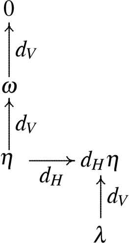
The relationship between ω, λ and η in Lemma 4.1 is represented by the diagram,
Corollary 4.4.
Let [ω] ∈ H1,2(ℛ∞) and let ω be a dV closed representative as in equation (4.10), and let λ ∈ Ω2,0(ℛ∞) be as in Lemma 4.1, so that dHη = dV λ. The linear map Λ : H1,2(ℛ∞) → H2,0(ℛ∞) given by
Proof.
Suppose ωa ∈ Ω1,2(ℛ∞), a = 1, 2 where [ω1] = [ω2] and that ωa = dV ηa, a = 1, 2 are dV closed representatives. Let λa ∈ Ω2,0(ℛ∞) satisfy dHηa = dV λa, a = 1, 2. To demonstrate [λ1] = [λ2] ∈ H2,0ℛ∞ we show there exists κ ∈ Ω1,0(ℛ∞) such that λ1 − λ2 = dHκ.
Since [ω1] = [ω2], there exists ξ ∈ Ω0,2(ℛ∞) such that,
Taking dV of equation (4.19) gives dV dHξ = −dHdV ξ = 0, which implies dV ξ = 0 since H0,2(ℛ∞) = 0 (or dHμ = 0, μ ∈ Ω0,s(ℛ∞) implies μ = 0). Therefore there exists ϕ ∈ Ω0,1(ℛ∞) such that ξ = dV ϕ. Substituting ξ = dV ϕ in equation (4.19) gives
The vertical exactness of the variational bicomplex applied to equation (4.20) implies that there exists κ ∈ Ω1,1(ℛ∞) such that
Taking dH of equation (4.21) and using dHηa = dV λa gives
Again by vertical exactness of the augmented variational bicomplex applied to equation (4.22), there exists μ ∈ Ω2,0(ℝ) such that
The relevance of the kernel of Λ is given in Theorem A.2.
5. Variational Operators and H1,2(ℛ∞)
A scalar evolution equation defined by the zero set of Δ = ut − K(t, x, u, ux, ..., un) is said to admit a variational operator of order k if there exists a differential operator
Theorem 5.1.
Let
With ı : ℛ∞ → J∞(ℝ2,ℝ) in equation (2.9) let,
Then dHω = 0.
Proof.
Suppose ℰ and L are given satisfying (5.1), then using the standard formula in the calculus of variations (for example equation (3.2) in [2]), we have on account of (5.1)
By applying ı* to equation (5.2) we have
Letting ω = dV ı* η, we compute dHω using equation (5.4) and get
Therefore dHω = 0.
A formula for ω in terms of ℰ in Theorem 5.1 is given in Theorem 5.2 below. Before giving Theorem 5.2 we note the following property of variational operators for evolutions equations.
Lemma 5.1.
If Δ = ut − K(t, x, u, ux, ..., un) admits the kth order variational operator
Proof.
Suppose ℰ(ut − K) = E(L) then applying I ∘ dV to equation (5.2) using
With Δ = ut − K let
In the term ∂ua,j ⌋ κ where κ is given in equation (5.6) we note that ∂ua,j (rj) = 0, ∂ua,j (K) = 0, a ≥ 1, j ≥ 0. Therefore the only possible non-zero terms in the summation term in equation (5.7) with ∂ua,j with a ≥ 1, j ≥ 0 satisfy
Writing the condition I(dt ∧ dx ∧ ϑ0 ∧ κ) mod {ϑ j}j≥0 using equation (5.7) and (5.8) gives
In order for the right side of equation (5.9) to be zero we must have ℰ* = −ℰ.
Theorem 5.2.
Let
Proof.
Let
Since
We now come to the last main theorem in this section which proves the converse to Theorem 5.1. The proof is again a generalization of the argument given in Theorem 2.6 of [7] for the multiplier problem.
Theorem 5.3.
Let [ω] ∈ H1,2(ℛ∞) with representative ω as in equation (4.10) of Theorem 4.2,
Let λ = Ldt ∧ dx satisfying dHη = dV λ from Lemma 4.1. Then
The proof requires considerable care whether we are working on ℛ∞ or J∞(ℝ2,ℝ), see Remark 2.1.
Proof.
We start by writing γ = gjθj in equation (5.12) and define the form
Since gj = gj(t, x, u, ux, ...) then W(gj) = 0, while
The condition dHη = dV λ (on ℛ∞) is
Now π*dt ∧ dx ∧ θj = dt ∧ dx ∧ ϑj (see Remark 2.1), and using the vector fields in (5.15) we have
Therefore applying π* to (5.18) and using (5.19) we have
The first variational formula for dV (Ldt ∧ dx) on J∞(ℝ2,ℝ) applied to the right side of (5.20) gives
The terms dV Δ · Q in equation (5.22) can be written as
We now apply the integration by parts operator (see equation 2.8 in [2]) and use the first variational formula for dV (QΔdt ∧ dx), in equation (5.23) and get
Next we expand the term V(Q) in equation (5.22) using V in (5.15) and
Inserting (5.24), and (5.25) into (5.22) and letting
This implies
Remark 5.1.
In general three applications of the vertical homotopy operator are required to determine λ ∈ Ω2,0(ℛ∞) from [ω] ∈ H1,2(ℛ∞). The first is to find a representative ω ∈ H1,2(ℛ∞) with dV ω = 0 (Theorem 4.2). The second is to find η such that dV η = ω, and the third is to find λ such that dV λ = dHη.
We now have the following corollaries.
Corollary 5.1.
Let [ω] ∈ H1,2(ℛ∞) with unique representative ω = dx∧θ0 ∧ɛ −dt ∧ β(ɛ), ɛ = riθi as in Theorem 4.1. Then Δ admits
Proof.
Starting with equation (5.12), Corollary 4.3 implies
Equation (5.26) together with the fact
Corollary 5.2.
Let [ω] ∈ H1,2(ℛ∞) with ω = dx∧ θ0 ∧ (riθi)−dt ∧ β(ρ) as in Theorem 3.1. Then Δ admits
Proof.
By Corollary 4.1 the unique representative
Corollary 5.3.
If an even order evolution equation ut = K(t, x, u, ..., u2m) m ≥ 1 admits a varia- tional operator ℰ, then ℰ = 0.
Proof.
Let ω ∈ Ω2,1(ℛ∞) be the dH closed form from Theorem 5.2. On the other hand using the representative for [ω] from Theorem 3.1 combined with Corollaries 3.1 and 5.2 implies ω = 0. Hence ℰ = 0.
Finally we may also restate Theorem 5.3 without reference to the equation manifold ℛ∞ as follows.
Corollary 5.4.
The operator
Lastly we combine the results of Theorems 5.1 and 5.3 to prove Theorem 1.1.
Proof.
(Theorem 1.1) We define a linear transformation
We check
Therefore Φ in equation (1.5) is invertible with
6. Functional 2-Forms, Symplectic Forms and Hamiltonian Vector Fields
In this section we review the space of functional forms on J∞(ℝ,ℝ) as in [3], [2] and relate these to symplectic forms, symplectic operators and Hamiltonian vector fields.
6.1. Functional Forms
On the space J∞(ℝ,ℝ) with coordinates (x,u,ux,...,ui,...) the contact forms are θi = dui −ui+1dx and Dx = ∂x +ux∂u +...ui+1∂ui +... is the total x derivative operator. Again Ωr,s(J∞(ℝ,ℝ)) denotes the r = 0,1 horizontal, s ≥ 0 vertical forms on J∞(ℝ,ℝ). The horizontal and vertical differentials dH : Ωr,s(J∞(ℝ,ℝ)) → Ωr+1,s(J∞(ℝ,ℝ)), dV : Ωr,s(J∞(ℝ,ℝ)) → Ωr,s+1(J∞(ℝ,ℝ)), are anti-derivations which satisfy
The integration by parts operator I : Ω1,s(J∞(ℝ,ℝ)) → Ω1,s(J∞(ℝ,ℝ)) is
The space of functional s forms (s ≥ 1) on J∞(ℝ,ℝ), ℱ s(J∞(ℝ,ℝ)) ⊂ Ω1,s(J∞(ℝ,ℝ)), is defined to be the image of Ω1,s(E) under I,
Equation (6.1) applied to Definition 6.3 shows that if Σ ∈ ℱ s(E) then there exists α ∈ Ω0,s−1(J∞(ℝ,ℝ)) such that
However, not every differential form Σ ∈ Ω1,s(J∞(ℝ,ℝ)) written in the form (6.4) is in the space ℱs(J∞(ℝ,ℝ)). In the case of ℱ 2(J∞(ℝ,ℝ)) the following is easy to show using the definition of I in (6.1), see also Proposition 3.6 and 3.7 in [3].
Lemma 6.1.
Let Σ ∈ ℱ 2(J∞(ℝ,ℝ)), then there exists a unique skew-adjoint differential operator,
The differential δV : ℱ s(J∞(ℝ,ℝ)) → ℱs+1(J∞(ℝ,ℝ)) is defined by
6.2. Symplectic Forms, Symplectic Operators, and Hamiltonian Vector Fields
Let Γ be the Lie algebra of prolonged evolutionary vector fields on J∞(ℝ,ℝ). We begin by recalling the appropriate definitions (see Section 2.5 [10]).
Definition 6.1.
An element Σ ∈ ℱ 2(J∞(ℝ,ℝ)) is a symplectic form on Γ if Σ ≠ 0 and δV (Σ) = 0. A skew-adjoint differential operator
Definition 6.1 combined with Lemma 6.1 shows there is a one-to-one correspondence between symplectic forms and symplectic operators. We now define Hamiltonian vector fields.
Definition 6.2.
Let Σ be a symplectic form. A vector field Y ∈ Γ is Hamiltonian if
The vector field Y is a degenerate direction if I(Y ⌋ Σ) = 0.
Definition 6.2 is equivalent to Σ being invariant under the flow of Y on ℱ 2(J∞(ℝ,ℝ)) as shown in the following theorem.
Theorem 6.1.
Let Σ be a symplectic form. An evolutionary vector field Y ∈ Γ is Hamiltonian with respect to Σ if and only if
Proof.
Using Lemma 3.24 in [3] and the fact that δV Σ = 0, we have
By the first property in equation (6.2), I ∘ dV ∘ I = I ∘dV, so conditions (6.7) and (6.8) are equivalent through equation (6.9).
We now write out definition 6.2 in a more familiar form. The exactness of the Euler complex and the condition δV ∘ I(Y ⌋ Σ) = 0 implies there exists λ = 2Hdx ∈ ℱ 0(J∞(ℝ,ℝ)) such that
Writing Y = pr(K∂u) and Σ = dx∧θ0 ∧𝒮(θ0) where
Using this computation in (6.10) shows that condition (6.7) (or (6.8)) is then equivalent to the following.
Corollary 6.1.
Let Σ be a symplectic form with corresponding symplectic operator 𝒮. The evolutionary vector field Y = pr(K∂u) ∈ Γ is Hamiltonian if and only if there exists H ∈ C∞(J∞(ℝ,ℝ)) such that
Corollary 6.1 just shows that Definition 6.2 agrees with the standard symplectic Hamiltonian formulation for time independent evolution equations [10].
6.2.1. Symplectic Potential
If Σ is a symplectic form, the exactness of the δV complex implies there exists ψ ∈ ℱ 1(J∞(ℝ,ℝ)) such that Σ = δV (ψ). The functional form ψ is a symplectic potential for Σ.
Lemma 6.2.
Let Σ ∈ ℱ 2(J∞(ℝ,ℝ)) be symplectic (and so δV closed), then there exists a smooth function P ∈ C∞(J∞(ℝ,ℝ)) such that
Proof.
A symplectic potential ψ ∈ ℱ1(J∞(ℝ,ℝ)) for Σ can be written using (6.4) as
Writing Σ = δV ψ and using equation (6.14) produces (6.13).
The Hamiltonian condition on Y ∈ Γ in terms of a symplectic potential ψ is the following.
Lemma 6.3.
The evolutionary vector field Y ∈ Γ is Hamiltonian for the symplectic form Σ = δV ψ if and only if there exists λ ∈ ℱ 0(J∞(ℝ,ℝ)) such that
Proof.
Using the exactness of the δV complex we show
Using either Lemma 6.3 or equations (6.13) and (6.1) we have the following simple corollary.
Corollary 6.2.
Let Σ be a symplectic form with symplectic potential ψ = dx∧θ0 ·P. The evolutionary vector field V = pr(K∂u) ∈ Γ is Hamiltonian if and only if there exists H ∈ C∞(J∞(ℝ,ℝ)) such that
A straight forward computation writing Σ = δV ψ classifies the first order symplectic operators, see also Theorem 6.2 in [10]
Lemma 6.4.
An element Σ ∈ ℱ 2(J∞(ℝ,ℝ)) of the first order form,
6.3. Time Dependent Systems
Most of the definitions and results from Sections 6.1 and 6.2 extend immediately to the case of time dependent systems. Let E = ℝ × J∞(ℝ,ℝ), and label the extra ℝ with the parameter t. The contact forms are
A generic form
The anti-derivations
The mapping
Lemma 6.5.
An element
We use Theorem 6.1 to define Hamiltonian vector fields in this case.
Definition 6.3.
An evolutionary vector field Y = pr(K∂u) where K ∈ C∞(E) is Hamiltonian with respect to the symplectic form
Note that T in Definition 6.3 agrees with T in equation (2.10). We can also write condition (6.23) as follows.
Lemma 6.6
An evolutionary vector field Y = pr(K∂u) is a Hamiltonian vector field for the symplectic form
Proof.
We have kernel
A formula for ξ in equation (6.24) in terms of
The analogue to Lemma 6.3 also holds in this case where Y is replaced by T. In order to prove this we now show the commutation formula in equation (6.16) holds where Y is replaced by T.
Lemma 6.7.
If
Proof.
Since T = ∂t +Y and
We write out both side of this equation. The left side is
The right side is
Since the mixed partials are equal Pt,i = Pi,t, equations (6.25) and (6.26) are equal, which proves the lemma.
Lemma 6.8.
The evolutionary vector field Y ∈ Γ is Hamiltonian for the symplectic form
Proof.
Using the exactness of the
Using Lemma 6.8 we have the following corollary which is the t-dependent version of Corollary 6.2.
Corollary 6.3.
Let
Proof.
We just need to compute
Using this computation in equation (6.27) with λ = 2Hdx gives equation (6.28).
The function H in (6.28) is the Hamiltonian.
Remark 6.1.
A symplectic form Σ is t-invariant if ℒ∂tΣ = 0. In this case Σ determines a well defined symplectic form
7. Variational and Symplectic Operator Equivalence
A time independent evolution equation ut = K(x,u,ux,...,un) is a symplectic Hamiltonian evolution equation [10] if there exists a symplectic operator 𝒮 and a function H called the Hamiltonian such that equation (1.6) holds. With this definition, the determination of the possible symplectic Hamiltonian evolution equations is typically approached in two ways. The first way consists of determining the possible symplectic operators of a certain order [10]. Then for a given class of symplectic operators 𝒮, determine K which satisfy equation (1.6). The second approach starts with a given K and then determines if there exists a symplectic operator 𝒮 such that equation (1.6) holds.
By comparison Theorem 1.3. whose proof is given in this section, combines these two questions and resolves the characterization of symplectic Hamiltonian evolution equations by the invariants H1,2(ℛ∞). This can simultaneously solve the existence of 𝒮 and the existence of the Hamiltonian function H in equation (1.6) as done for the special case given in Theorem 1.4.
7.1. H1,2(ℛ∞) and Symplectic Hamiltonian Evolution Equations
Given a scalar evolution equation ut = K(t, x, u, ux, ...), we identify the manifolds ℛ∞ and E = ℝ × J∞(ℝ,ℝ) by identifying their coordinates which in turn induces an identification of smooth functions. Define the projection map Π : T*(ℛ∞) → T*(E) by
Lemma 7.1.
The map
Proof.
Equation (7.3) follows for the case ω = θi directly from equations (2.15) and (6.20), and generically from the anti-derivation property of the operators.
Lemma 7.2.
The function
Proof.
To show
Therefore
We now show
Since dV ω ∈ H1,3(ℛ∞), Theorem 3.2 implies there exists ξ ∈ Ω0,3(ℛ∞) such that dV ω = dHξ so equation (7.5) becomes
Therefore
We now show
In particular we have
Corollary 7.1.
If [ω] ≠ 0 then
We now set out to prove the fact that
Lemma 7.3.
Let si,ξij ∈ C∞(ℛ∞) then
Proof.
Since
We now have the main theorem.
Theorem 7.1.
Let
Proof.
Supposed Σ is symplectic and Y is Hamiltonian, then Lemma 6.6 produces
Equations (7.6) and (6.24) give
Therefore [ω] ∈ H1,2(ℛ∞). Now Theorem 3.4 implies ξabθ a ∧ θb = −β (siθi) so that ω in equation (7.8) and equation (7.7) are the same.
Suppose now that ω in equation (7.7) is dH closed. By Lemma 7.2,
Writing β (siθi) = Babθ a ∧ θb and using equations (7.6) we have
This will vanish if and only if
We now summarize the results of Lemma 7.2 and Theorem 7.1 by the following corollary.
Corollary 7.2.
Let ut = K be an evolution equation, and let Y = pr(K∂u) be the corresponding evolutionary vector field on E and let
With Theorem 1.1 and Corollary 7.2 in hand the proof of Theorem 1.2 and 1.3 are now easily given.
Proof.
(Theorems 1.2 and 1.3) We start with Theorem 1.2 and suppose that
To prove Theorem 1.3 we identify as above, a symplectic operator 𝒮 on E as an operator on J∞(ℝ2,ℝ) (see Remark 2.1). The function Φ in equation (1.5) defines an isomorphism between symplectic operators for Δ and H1,2(ℛ∞). This proves Theorem 1.3.
As our final Lemma we show for completeness how formula (5.13) can be determined from the symplectic potential.
Lemma 7.4.
Let
Proof.
By equation (7.11) of Corollary 7.2 we have the unique representative as stated in the lemma.
We prove the second part of the lemma by first using Theorem 4.2 to construct a representative ω0 for Ψ(𝒮) such that ω0 = dV η0 with η0 = dx∧ θ0 ·Q−dt ∧ γ0. By equation (4.17) of Corollary 4.3 and equation (6.22) for the operator in the form ɛ = 𝒮(θ0) gives
Lemma 6.5 and equation (7.13) show
7.2. Time Independent Operators
Equation (1.6) defines when the time independent evolution equation ut = K(x, u, ux, ...) is a Hamiltonian evolution equation with symplectic operator 𝒮. This is precisely the same definition that the ordinary differential equation K(x, u, ux, ...) = 0 admits 𝒮 as a variational operator. The following simple lemma is the key to decoupling the variational operator problem for time independent scalar evolution equations.
Lemma 7.5.
Let 𝒮 = siDxi be a time independent symplectic operator with symplectic potential P ∈ C∞(J∞(ℝ,ℝ)) (equation (6.13) in Lemma 6.2). Then
Proof.
By the product formula in the calculus of variations (equation 5.80 in [17]) the left side of equation (7.16) is
Equation (7.17) together with the fact from equation (6.13) that
We then have the following.
Theorem 7.2.
Let 𝒮 be a t-independent symplectic operator. The following are equivalent,
- (1)
ut = K(x, u, ux, ..., u2m+1), m ≥ 1, satisfies 𝒮(K) = E(H).
- (2)
𝒮 is a symplectic variational operator for the ODE K = 0,
- (3)
𝒮 is a variational operator for ut = K (see Remark 2.1).
This converts the symplectic Hamiltonian question for the evolution equation into a variational operator problem for the ODE K = 0.
Proof.
Suppose ut = K(x, u, ..., u2m+1) is Hamiltonian for the t-independent symplectic operator 𝒮, so that 𝒮(K) = E(H) on J∞(ℝ,ℝ). By definition 𝒮 is a variational operator for the ODE K = 0. So (1) and (2) are trivially equivalent.
We show (1) implies (3). Suppose that 𝒮(K) = E(H). Using equation (7.17) in Lemma 7.5 we have
Finally we show (3) implies (1). Lemma 7.4 which allows Q in equation (5.13) to be replaced with the symplectic potential P so that hypothesis (3) implies,
Substituting from equation (7.17) into equation (7.18) we get
Therefore
It is worth noting that if [ω] ∈ H1,2(ℛ∞) then [∂t ⌋ ω]K=0 ∈ H1,2(K = 0) [5]. That is, in the time independent case, the form β in Lemma 3.2 (restricted to the ODE K = 0) defines an H0,2 cohomology class for the ODE K = 0.
8. First Order Operators and Hamiltonian Evolution Equations
8.1. First Order Operators for Third Order Equations
For a third order evolution equation
Proof.
(Theorem 1.4) By Theorem 1.1 and Corollary 4.2 the skew-adjoint operator ℰ = 2RDx + X(R) is a variational operator for (8.1) if and only if the skew-adjoint form
The highest possible θi ∧ θ0 term in equation (8.2) using (8.3) is θ4. We find from equation (8.2)
While for θ3 ∧ θ0, θ2 ∧ θ0 and θ1 ∧ θ0 we have from equations (8.3) and (8.2),
For the coefficient of θ3 ∧ θ0 to be zero we have from equation (8.4),
Simplifying equation (8.6) using equation (8.5) we get
It follows that a non-vanishing R (which we may assume to be positive) satisfying equations (8.5) and (8.7), which is necessary and sufficient for the existence of a first order variational operator for Δ = ut − K in equation (8.1), is equivalent to A = X(logR) and B = T(logR) satisfying the conditions in Theorem 1.4. This proves Theorem 1.4.
The form κ in equation (1.7) for the KdV equation ut = uxxx + uux satisfies
Therefore according to Theorem 1.4 there is no first order formulation for the KdV equation as a symplectic Hamiltonian evolution equation.
8.2. First Order Hamiltonians Operators and their Potential Form
Let vt = 𝒟 ∘ E(H(x,v,vx,...)) be a time independent Hamiltonian evolution equation where 𝒟 is a first order Hamiltonian operator. According to [16] or [1] we may choose coordinates (using a contact transformation) such that 𝒟 = Dx. The following is Theorem 1 in [15] in the context of scalar evolution equations.
Lemma 8.1.
The potential form of the Hamiltonian evolution equation,
Equation (8.9) admits ℰ = Dx as a first order variational operator, and satisfies
There is an abuse of notation in this lemma where Dx is used as the total x derivative operator in either variable u or v depending on context.
Proof.
Starting with equation (8.8), let v = ux so that (8.8) becomes
Integrating equation (8.11) with respect to x gives the potential form (8.9).
To prove equation (8.10) holds, we simply need the change of variables formula, see exercise 5.49 in [17],
Equation (8.12) together with the simple fact −2E(utux) = utx proves equation (8.10).
The second term in the right hand side of equation (8.10) is just the pullback of the Hamiltonian function in (8.8). We also note the following simple corollary.
Corollary 8.1.
Every Hamiltonian evolution equation vt = 𝒟(E(H1(x, v, vx, ...))) with first order Hamiltonian operator 𝒟 is the symmetry reduction of an equation ut = K(x, u, ux, ...), of the same order, which admits an invariant first order variational operator.
8.3. Bi-Hamiltonian Evolution Equations with a First Order Hamiltonian Operator
We now present sufficient conditions when the potential form of a compatible bi-Hamiltonian system admits another variational operator.
Theorem 8.1.
Let vt = K(x, v, vx, ...) = Dx (E(H1(x,v,vx,...))) be a Hamiltonian evolution equation with potential form
Let 𝒟0 be second time independent Hamiltonian operator with Hamiltonian H0(x, v, vx, ...) satisfying,
Assume 𝒟0 also satisfies the compatibility condition (equation 7.29 in [17])
Then the right hand side of the potential form satisfies
Proof.
First we apply ℰ = 𝒟0|v=ux to the right hand side of equation (8.13), and use condition (8.14) to get
Again the last line follows from the change of variables formula in the calculus variations (exercise 5.49 in [17]). This verifies equation (8.15). Then by part (1) of Theorem 7.2 equation (8.15) shows that ℰ is a variational operator for equation (8.13). If Q is the function from equation (5.28) we then have
Theorem 8.1 makes the hypothesis that ℰ = 𝒟0|v=ux is a symplectic operator. This holds in the case of the Hamiltonian operators given by Theorem 5.3 in [10],
9. Examples
Example 9.1.
The Harry-Dym equation zt = z3zxxx [10,21] is a compatible bi-Hamiltonian system,
The change of variable z = v−1 maps the Hamiltonian operator
The Harry-Dym equation (9.1) in these coordinates is then,
The potential form of equation (9.4) is found by letting v = wx and integrating to get (see also (8.9))
Equation (8.10) of Lemma 8.1 as it applies to the potential Harry-Dym equation (9.5) produces the following variational operator equation for Dx,
We now apply Theorem 8.1 to obtain a second variational operator. The compatibility condition in equation (8.14) is satisfied with the operators from equation (9.3) with
The operator 𝒟0 in equation (9.3) is of the form (8.19) so that by equation (8.20)
Equation (8.16) with Q in equation (9.8) and H2 in equation (9.6) (with v = wx) gives the variational operator equation for the potential Harry-Dym equation (9.5),
If we return to the original coordinates for the Harry-Dym equation and make the change of variable given by x = u, w = x,
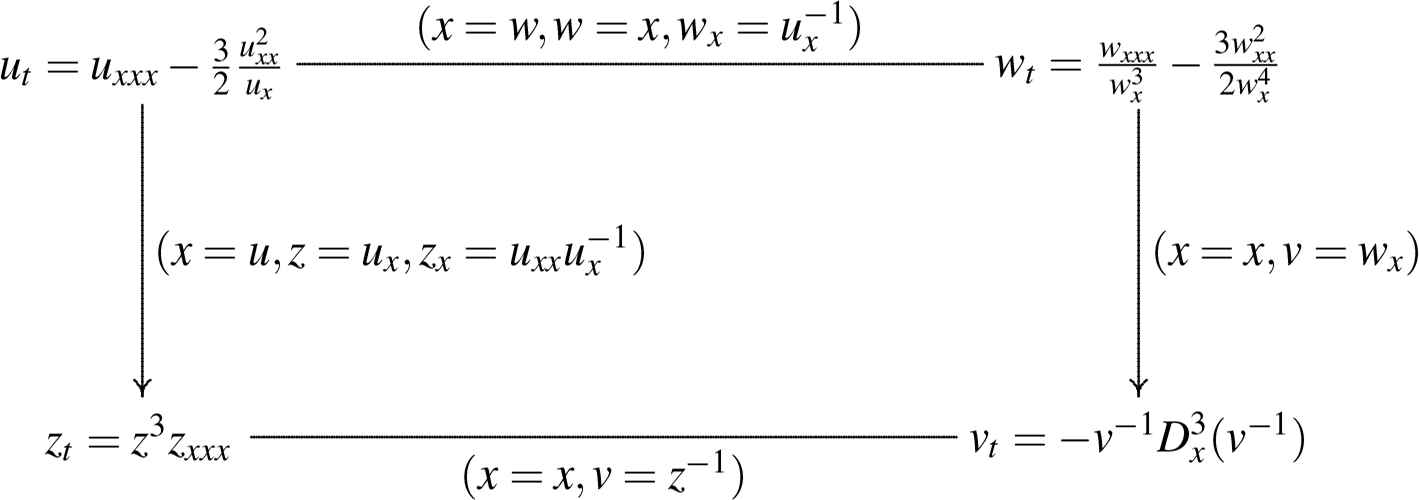
In particular the Krichever-Novikov in equation (9.9) is the potential form of the Harry-Dym equation (9.1). These different coordinate representations of the Harry-Dym equation and the Krichever-Novikov equation is summarized by the diagram,
 (9.10)
The variational or symplectic operators for the Krichever-Novikov equation are obtained by applying the change of variables x = u,w = x,
With quotient map
We now compute the explicit unique representative for the H1,2(ℛ∞) cohomology class for the Krichever-Novikov equation (9.9) corresponding to the first operator in (9.11) (Theorem 4.1). This is computed using formula (1.4) in Theorem 1.1 to be,
We have dV ω1 = 0 and for the forms η and λ in Theorem 5.3 we may choose
Likewise formula (1.4) for the second operator in (9.11) gives the unique cohomology representative (Theorem 4.1),
In this case
For λi in equations (9.13) and (9.16), it is difficult to determine whether [λi] ∈ H2,0(ℛ∞) is trivial or not (see Theorem A.2). However, it is possible but not easy to show λi ≠ dκi where κi is t-invariant by using the infinite sequence of conservation laws [10] for the Krichever-Novikov (Schwarzian KdV) equation (9.9). The forms λi define a non-trivial cohomology class in the t-invariant variational bi-complex for (9.9).
Example 9.2.
The Harry Dym equation can be written in the form
Equation (9.17) is obtained from equation (9.4) by substituting
Another potential form (or integrable extension) for the Harry-Dym equation (9.17) can be obtained by letting v = uxxx in equation (9.17) so that
We show that
The operator
In equation (8.14) compatibility was used to show the second Hamiltonian operator for a bi-Hamiltonian equation became a variational operator for the potential form. In order to use a similar argument in this case we need to show 𝒟1E(H0) = 𝒟0E(H−1). We find
In analogy to equation (8.14), this gives rise with H−1 = 0 to the variational operator
Using the fact that operator ℰ in equation (9.21) is a symplectic operator, the compatibility condition (9.20) gives
Equation (9.22) shows directly that ℰ in (9.21) is a variational operator for equation (9.18).
It is worth noting that ℰ(K) = 0 in this example and that [ω] = dV [η] where [η] ∈ H1,1(ℛ∞). The representative
Since dHη = 0, [η] ∈ H1,1(ℛ∞). This also produces an example where
Example 9.3.
The cylindrical KdV equation is (see [21])
The form κ in equation (1.7) in Theorem 1.4 is κ = t−1dt = dH(logt) and so equation (9.24) admits ℰ1 = tDx as a variational operator. In equation (5.13) we have
Note that the Lagrangian on the right side of this equation differs from that in equation (1.3) by a total divergence.
By solving the equation
For ℰ0 we have
If we now compute the reduction of the potential cylindrical KdV by substituting
Equation (9.25) can of course be obtained from the cylindrical KdV equation (9.23) by the change of variables
More generally any evolution equation of the form
For the + sign in equation (9.28), the change of variables
10. Conclusions
The determination of a variational or symplectic operator for a scalar evolution equation has been shown to be equivalent to the non-vanishing of a cohomology class in H1,2(ℛ∞). The arguments used to prove this clearly extend to other types of differential equations including systems. For example Theorem 5.1 holds independently of Δ being a evolution equation and so the variational operators for Δ always determine an element of the cohomology Hn−1,2(ℛ∞) as in Theorem 5.1.
There remain many open theoretical questions such as how the compatibility condition for symplectic operators appears in the cohomology. Another interesting problem is to determine under what conditions the symmetry reduction of a variational operator equation is a Hamiltonian system (the converse of Lemma 8.1).
Many difficult computational questions have also not been resolved. We were unable to compute the dimension of H1,2(ℛ∞) in our examples. Preliminary computations using equation
A. The Vertical Differential
The vertical differential induces a mapping dV : Hr,s(ℛ∞) → Hr,s+1(ℛ∞) defined by dV [ω] = [dV ω]. Let ut = K be a scalar evolution equation with equation manifold ℛ∞. We now examine when [ω] ∈ ImagedV .
Theorem A.1.
Let [ζ] ∈ H1,1(ℛ∞). There exists [κ] ∈ H1,0(ℛ∞) such that [ζ] = dV [κ] if and only if δV ∘ Π(ζ) = 0 where
This answers the question of when [ζ] is the image of a classical conservation law [κ]. To relate Theorem A.1 to the theory of characteristics for a conservation law, suppose [ζ] ∈ H1,1(ℛ∞) with (unique) canonical representative given in Theorem 3.3 by
Proof.
Suppose [ζ] ∈ H1,1(ℛ∞) where ζ = dx ∧ (aiθi) − dt ∧ β is a representative, then
This implies by equation (6.2),
Let μ = miθi ∈ Ω1,0(ℛ∞) and
Therefore there exists
Now
However dV β ∈ Ω0,2(ℛ∞) and the only way the contact two form dV β satisfies equation (A.4) is if dV β = 0. This implies from equation (A.3) that
Using the vertical exactness of Ω1,1(ℛ∞) we conclude there exists κ ∈ Ω1,0(ℛ∞) such that
Again by vertical exactness of the (augmented) variational bicomplex for dV : Ω2,0(ℛ∞) → Ω2,1(ℛ∞) applied to dHκ we have,
Since ℝ2 is simply connected we may write
Finally let
Therefore
Corollary A.1.
Let [ζ] ∈ H1,1(ℛ∞) with canonical representative given by
Corollary A.2.
If ut = K(t, x, u, ..., u2m), m ≥ 1 is even order, then every solution Q to
As is well known, the characteristic of a conservation law is a solution to
We now examine the case of H1,2(ℛ∞).
Theorem A.2.
Let [ω] ∈ H1,2(ℛ∞). Then [ω] = dV [η] where [η] ∈ H1,1(ℛ∞) if and only if [ω] ∈ KerΛ where Λ : H1,2(ℛ∞) → H2,0(ℛ∞) is defined in equation (4.18).
Proof.
Let [ω] ∈ H1,2(ℛ∞) with representative ω satisfying ω = dV η and λ be as in Lemma 4.1. That is
Suppose now that λ = dHκ so that [ω] ∈ KerΛ. Let
Therefore
Suppose now that [ω] = dV [η] where [η] ∈ H1,1(ℛ∞). Let ω be the representative such that ω = dV η. By hypothesis dHη = 0 and so for λ in Lemma 4.1 we have
The same argument as in the second part of the proof of Corollary 4.4 implies that there exists κ ∈ Ω1,0(ℝ2) such that λ = dHκ. Therefore Λ([ω]) = [λ] = [dHκ] = 0.
Theorem A.2 is demonstrated in Example 9.2. As a simple corollary to Theorem A.2 we can identify the elements of H1,1(ℛ∞) which are not the image of a conservation law as follows.
Corollary A.3.
The map dV : H1,1(ℛ∞)/dV (H1,0(ℛ∞)) → KerΛ is an isomorphism. Moreover, we can identify η ∈ H1,1(ℛ∞)/dV (H1,0(ℛ∞)) with the space of functions Q ∈ C∞(ℛ∞) such that
Footnotes
𝒟0 is the push-forward of ℰ by the quotient map q : (t,x,u,ux,...) → (t, x, v, vx, ...).
References
Cite this article
TY  - JOUR
AU  - M.E. Fels
AU  - E. Yaşar
PY  - 2019
DA  - 2019/07/09
TI  - Variational Operators, Symplectic Operators, and the Cohomology of Scalar Evolution Equations
JO  - Journal of Nonlinear Mathematical Physics
SP  - 604
EP  - 649
VL  - 26
IS  - 4
SN  - 1776-0852
UR  - https://doi.org/10.1080/14029251.2019.1640470
DO  - 10.1080/14029251.2019.1640470
ID  - Fels2019
ER  -