A New Zero-Truncated Version of the Poisson Burr XII Distribution: Characterizations and Properties

Haitham M. Yousof; Mohammad Ahsanullah; Mohamed G. Khalil

doi:10.2991/jsta.d.190306.001

Download article (PDF)

Next Article In Issue>

Volume 18, Issue 1, March 2019, Pages 1 - 11

A New Zero-Truncated Version of the Poisson Burr XII Distribution: Characterizations and Properties

Authors

Haitham M. Yousof¹^{, *}, Mohammad Ahsanullah², Mohamed G. Khalil¹

¹Department of Statistics, Mathematics and Insurance, Benha University, Benha, Egypt

²Department of Management Sciences, Rider University, New Jersey, USA

^*Corresponding author. Email: haitham.yousof@fcom.bu.edu.eg

Corresponding Author

Haitham M. Yousof

Received 13 July 2018, Accepted 10 February 2019, Available Online 22 April 2019.

DOI: 10.2991/jsta.d.190306.001 How to use a DOI?
Keywords: Zero-truncated Poisson; Poisson Topp Leone; Burr XII distribution; simulation; characterizations
Abstract: In this work, a new four-parameter zero-truncated Poisson Topp Leone Burr XII distribution is defined and studied. Various structural mathematical properties of the proposed model including ordinary and incomplete moments, residual and reversed residual life functions, generating functions, order statistics are investigated. Some useful characterizations are also presented.
Copyright: © 2019 The Authors. Published by Atlantis Press SARL.
Open Access: This is an open access article distributed under the CC BY-NC 4.0 license (http://creativecommons.org/licenses/by-nc/4.0/).

1. INTRODUCTION

The Pearson system of frequency curves was introduced by Pearson [1] who worked out a set of four-parameter probability density functions (PDFs) as solutions to the following differential equation

f′x/fx=Px/Qx=x−ab0+b1x+b2x2−1

where f is a density function and a,b0,b1, and b2 Pearson family such as Gamma, Gaussian, Beta, and Student's t models. Analogously to the Pearson system, Burr [2] introduced another system of frequency curves that includes 12 types of cumulative distribution functions (CDFs) which yield a variety of density shapes, this system is obtained by considering CDFs satisfying a differential equation which has a solution, given by

Gx=1+exp−∫τxdx−1,

where τx is chosen such that Gx is a CDF on the real line and has 12 choices which made by Burr, resulted in 12 models which might be useful for modeling data, the principal aim in choosing one of these forms of distributions is to facilitate the mathematical analysis to which it is subjected, while attaining a reasonable approximation. A special attention has been devoted to one of these forms denoted by type XII (for more details see Burr [2–4], Burr and Cislak [5], Hatke [6], and Rodriguez [7]), whose CDF, Gx, is given as

Gα,βx=1−1+xα−β,

where both α and β are shape parameters. The location and scale parameters can easily be introduced to make Gα,βx a four-parameter distribution. The corresponding PDF is given by

gα,βx=αβxα−11+xα−β−1.

The Burr XII (BXII) (see Burr [2]) has many applications in different areas including reliability, acceptance sampling plans, and failure time modeling. Tadikamalla [8] studied the BXII model and its related models. Zimmer et al. [9] proposed a new three-parameter BXII distribution, this distribution, having the Weibull and the logistic as submodels, is a very popular distribution for modeling lifetime data and phenomenon with monotone failure rates. Shao [10] studied the maximum likelihood estimations for the three-parameter BXII model then Soliman [11] studied the estimation of parameters of life from progressively via censored data using Burr-XII model, Wu et al. [12] discussed the estimation problems for BXII model on the basis of progressive type II censoring under random removals where the number of units removed at each failure time has a discrete uniform model. Recently, Silva et al. [13] introduced the log-BXII regression models with censored data, Silva et al. [13] proposed a new location-scale regression model based on BXII model, Silva et al. [14] proposed a residual for the log-BXII regression distribution whose empirical model is close to normality, Afify et al. [15] studied the Weibull BXII distribution, Cordeiro et al. [16] proposed the double BXII model among others. For the other new extensions of the BXII see Altun et al. [17], Altun et al. [18], Paranaíba et al. [19], Yousof et al. [20], and Yousof et al. [21].

The rest of the paper is outlined as follows. In Section 2, we introduce the new model and its physical motivation. Section 3 presents some plots and the justification for introducing the new model. Some useful characterizations are presented in Section 4. In Section 5, we derive some statistical properties for the new model. Finally, we offer some concluding remarks in Section 6.

2. THE NEW MODEL AND ITS PHYSICAL MOTIVATION

The CDF and the PDF of the Topp Leone BXII (TLBXII) distributions (Reyad and Othman [22]) are given by

(1)Hb,α,βx=1−1+xα−2βb

and

(2)hb,α,βx=2bαβxα−11+xα−2β−11−1+xα−2βb−1

respectively. Suppose Z1,Z2,…,ZN be independent identically random variable (iid rv) with common CDF of the TLBXII model and N be a rv with probability mass function (PMF)

PN=n=an/ea−1n!| n=1,2,…, a>0

and define

MN=maxZ1,Z2,…,ZN

then

(3)Fx=∑n=0∞pMN≤x|N=npN=n

As described in Ramos et al. [23], Eq. (3) can be expressed as

(4)F(x)=∑n=1∞ 1ea−1ann!1−(1+xα)−2βbn

Using Eqs. (2) and (4), we can write

(5)Fx=1−exp−a1−1+xα−2βb/1−e−a.

Equation (5) is the CDF of the zero-truncated Poisson Topp Leone BXII (ZTPTLBXII) model. Henceforward fx=fa,b,α,βx and Fx=Fa,b,α,βx. The corresponding PDF of Eq. (5) reduces to

(6)fx=2abαβ1−e−axα−11+xα−2β−11−1+xα−2βb−1exp−a1−1+xα−2βb︸A.

Now we can provide a useful linear representation for the ZTPTLBXII density function in Eq. (6). Expanding the quantity A in power series, we can write

(7)fx=∑i=0∞2−1iai+1bαβi!1−e−axα−11+xα−2β−11−1+xα−2βbi+1−1.

Consider the power series

(8)1−ζτ−1=∑r=0∞−1rΓτζr/j!Γτ−j=∑r=0∞−1rτ−1 rζr,

which holds for |ζ|<1 and τ>0 real non-integer. Using the power series in Eq. (8) and after some algebra the PDF of the ZTPTLBXII model in Eq. (7) can be expressed as

fx=∑i=0∞2−1iai+1bαβi!1−e−axα−11+xα−2β−11−1+xα−2βbi+1−1=∑i,r=0∞2−1i+rai+1bi!1−e−aαβxα−11+xα−2β−11+xα−2rβbi+1−1r=∑i,r=0∞2−1i+rai+1bi!1−e−abi+1−1rαβxα−11+xα−2β1+r−1=∑i,r=0∞2−1i+rai+1bi!1−e−a21+rbi+1−1rα21+rβxα−11+xα−2β1+r−1=∑r=0∞∑i=0∞−1i+rai+1bi!1−e−a1+rbi+1−1r︸vrα21+rβxα−11+xα−21+rβ−1︸gα,21+rβx=∑r=0∞vrgα,21+rβx,

where

gα,21+rβx=2α1+rβxα−11+xα−21+rβ−1,

is the BXII density with parameters α and 21+rβ.

vr=∑i=0∞−1i+rai+1bi!1−e−a1+rbi+1−1 r

Via integrating Eq. (9), we obtain the same mixture representation

(9)Fx=∑r=0∞vrGα, 21+rβx,

where Gα, 21+rβx is the CDF of the BXII density with parameters α and 21+rβ. The new model has a wide application in many types of data such as Guinea pigs (Bjerkedal [24]) and many other data types.

3. PLOTS AND JUSTIFICATION

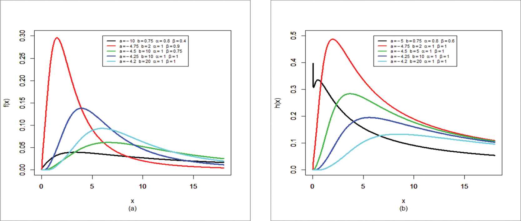
In this section, we provide some graphical plots of the PDF and hazard rate function (HRF) of the ZTPTLBXII model to show its flexibility. Figure 1(a) displays some plots of the ZTPTLBXII density for some parameter values a,b,α, and β. Plots of the HRF of the ZTPTLBXII model for selected parameter values are given in Fig. 1(b), where the HRF can be upside down bathtub (unimodal) and decreasing.

The justification for introducing the ZTPTLBXII lifetime model is based on the wider use of the BXII model. As well as we are motivated to introduce the ZTPTLBXII lifetime model because it exhibits the unimodal hazard rate as illustrated in Fig. 1(b). It is shown above that the ZTPTLBXII lifetime model can be viewed as a linear mixture of the BXII densities as illustrated in Eqs. (9) and (10).

4. CHARACTERIZATIONS

We will need the following two Lemmas for the characterization of the distribution:

Assumption A.

X is an absolutely continuous rv with CDF Fx and PDF fx. We assume EX exists and fx is differentiable. We assume further

α=supx | fx>0 and βx|fx<1.

Lemma 1.

If

EX | X≤x=gxfx/Fx,

where gx is a continuous differentiable function in α,β, then fx=cexp∫x−g′xgxdx, c is determined by the condition ∫αβfxdx=1.

Proof.

gx=∫αxufudufx, thus ∫αxufudu=fxgx

Differentiating both sides of the above equation, we obtain xfx=f′xgx+fxg′x on simplification, we get

f′x/fx=x−g′x/gx.

On integrating both sides of the above equation, we obtain

fx=cexp∫x−g′xgxdx,

where c is determined by the condition

∫αβfxdx=1.

Lemma 2.

Under the assumption A, if

EX | X≥x=hxfx/1−Fx,

where hx is a continuous differentiable function in α,β, then

fx=cexp∫=x+h′xhxdx,

where c is determined by the condition ∫αβfxdx=1.

Proof.

hx=∫x∞ufudufx, thus ∫x∞ufudu=fxhx

Differentiating both sides of the above equation, we obtain −xfx=f′xhx+fxh′x on simplification, we obtain

f′x/fx=−x+h′x/hx.

On integrating both sides of the above equation, we obtain

fx=cexp∫−x+h′xhxdx,

where c is determined by the condition

∫αβfxdx=1.

Theorem 1.

Suppose that the random variable X satisfies the conditions of the assumption A with α=0 and β=∞. Then, EX|X≤x=gxτx, where τx=fxFx and

gx=∑r=0∞νr21+rβBxα,1+1α,21+rβ−1α∑r=0∞νrgα,21+rβx,

if and only if

fx=∑r=0∞νrgα,21+rβx.

Proof.

Suppose that

fx=∑r=0∞νrgα,21+rβx,

then

fxgx=∑r=0∞νr∫0xugα,21+rβudu=∑r=0∞νr∫0x2α1+rβuα1+uα−21+rβ−1du=∑r=0∞νr∫0xα21+rβ1+tβ21+rβ−1t1αdt=∑r=0∞νr21+rβB1+1α,21+rβ−1α.

Thus

gx=∑r=0∞νr21+rβBxα,1+1α,21+rβ−1α∑r=0∞νrgα,21+rβx.

Suppose

gx=∑r=0∞νr21+rβBxα,1+1α,21+rβ−1α∑r=0∞νrgα,21+rβx,

then

g′x=x−∑r=0∞νr21+rβBxα,1+1α,21+rβ−1α∑r=0∞νrgα,21+rβx×∑r=0∞νr2α1+rβxα−2α−1−2αβ1+r+1xα1+xα21+rβ+2∑r=0∞νrgα,21+rβx=x−gx∑r=0∞νrα21+rβxα−2α−1−2αβ1+r+1xα1+xα21+rβ+2∑r=0∞νrgα,21+rβx

Thus

x−g′xgx=∑r=0∞νr2α1+rβxα−2α−1−2αβ1+r+1xα1+xα21+rβ+2∑r=0∞νrgα,21+rβx.

By Lemma 1, we have

f′xfx=∑r=0∞νrα1+rβxα−2α−1−2αβ1+r+1xα1+xα21+rβ+2∑r=0∞νrgα,21+rβx.

Integrating both sides of the above equation we obtain

fx=c∑r=0∞νrgα,21+rβx,

where c is constant. Using the condition ∫0∞fxdx=1, we obtain

fx=∑r=0∞νrgα,21+rβx.

Theorem 2.

Suppose that the random variable X satisfies the conditions of the assumption A with α=0 and β=∞.

Then, EX|X≥x=hxrx, where rx=fxFx and

gx=∑r=0∞νr21+rβBcxα,1+1α,β−1α∑r=0∞νrgα,21+rβx,

if and only if

fx=∑r=0∞νrgα,1+rβx,

where

Ba1,a2=∫0∞ta1−11+t−a1+a2dt

and

Bz,a1,a2=∫0zta1−11+t−a1+a2dt

are the beta and the incomplete beta functions of the second type, respectively.

Proof.

Suppose that fx=∑r=0∞νrgα,21+rβx, then

fxgx=∑r=0∞νr∫x∞ugα,21+rβudu=∑r=0∞νr∫x∞2α1+rβuα1+uα−21+rβ−1du=∑r=0∞νr∫x∞21+rβ1+t−21+rβ−1t1αdt=∑r=0∞νr21+rβBc1+1α,21+rβ−1α.

Thus

g(x)=∑r=0∞vr2(1+r)βBc1+1α, 2(1+r)β−1α∑r=0∞vrgα, 2(1+r)β(x).

Suppose

g(x)=∑r=0∞νr2(1+r)βBc(1+1α, 2(1+r)β−1α)∑r=0∞νrgα, 2(1+r)β(x),

then

g′x=−x−∑r=0∞νr21+rβBxα,1+1α,21+rβ−1α∑r=0∞νrgα, 21+rβx×∑r=0∞νr2α1+rβxα−2α−1−2αβ1+r+1xα1+xα21+rβ+2∑r=0∞νrgα,21+rβx=−x−gx∑r=0∞νrα21+rβxα−2α−1−2αβ1+r+1xα1+xα21+rβ+2∑r=0∞νrgα,21+rβx

Thus

x−g′(x)g(x)=∑r=0∞νr2α(1+r)βxα−2α−1−2αβ(1+r)+1xα(1+xα)2(1+r)β+2∑r=0∞νrgα,(1+r)β(x).

By Lemma 2, we have

f′(x)f(x)=∑r=0∞νrα(1+r)βxα−2α−1−2αβ(1+r)+1xα(1+xα)2(1+r)β+2∑r=0∞νrgα, 2(1+r)β(x).

Integrating both sides of the above equation we obtain

fx=c∑r=0∞νrgα, 2(1+r)βx,

where c is constant. Using the condition

∫0∞fxdx=1,

we obtain fx=∑r=0∞νrgα, 2(1+r)βx.

5. MATHEMATICAL PROPERTIES

5.1. Moments and Incomplete Moments

The rth ordinary moment of X is given by

μn′=EXn=∫−∞∞xnfxdx.

Then we obtain

(10)μr′=∑r=0∞vr∫0∞xngα, 21+rβx=∑r=0∞vr21+rβB1+nα,21+rβ−nα.

By setting n=1 in Eq. (11), we have the mean of X. The sth incomplete moment, say Ist, of X can be expressed from (9) as Ist=∫−∞txsfxdx. Then

(11)Ist=∑r=0∞vr∫−∞txs gα, 21+rβ(x)dx=∑r=0∞vr21+rβBtα;1+sα,21+rβ−sα,

The general equation for the first incomplete, I1t, can be derived from Eq. (12) as

I1t=∑r=0∞vr∫−∞tx gα, 21+rβxdx=∑r=0∞vr21+rβBtα;1+1α,21+rβ−1α.

5.2. Moment Generating Function

The moment generating function (MGF) of X, say MXt=EexptX, can be obtained from Eq. (9) as MXt=∑r=0∞vrM21+rβt, where M21+rβt is the mgf of the BXII distribution with parameters α, 21+rβ, then we have

MXt=∑r=0∞vrMr+1t=2αβ∑r=0∞1+rvr∫0∞exptxxα−11+xα−21+rβ−1dx=2αβ∑r=0∞1+rvr∑k=0∞tkk!∫0∞xα+k−11+xα−21+rβ−1dx.

Let u=xα, then

MXt=2β∑r=0∞1+rvr∑k=0∞tkk!∫0∞ukα1+u−21+rβ−1du=2β∑r=0∞1+rvr∑k=0∞tkk!B1+nα,21+rβ−nα,

which also means that the rth ordinary moment of X is

μr′=2β∑r=0∞vr1+rB1+nα,21+rβ−nα.

5.3. Order Statistics

Let X1,…,Xn be a random sample from the ZTPTLBXII model of distributions and let X1 : n,…,Xn : n be the corresponding order statistics. The PDF of ith order statistic, say Xi : n, can be written as

(12)fi : nx=Bi,n−i+1−1∑j=0n−i−1jn−i jfxFj+i−1x,

where B⋅,⋅ is the beta function. Substituting Eqs. (5) and (6) in Eq. (13) and using a power series expansion, we get that

fxFxj+i−1=∑h=0∞vhgα,1+hβx,

where

vh=∑w,m,k=0∞2bw+1−mbaw+1−1w+m+k+hk+1ww!h!1+h1−e−aj+ij+i−1 kbw+1−1 m×1+βw+1+m h−2+βw+1+m h

The PDF of Xi : n can be expressed as

fi : nx=∑j=0n−i−1jn−i jBi,n−i+1−1∑h=0∞vhgα,1+hβx.

For example, the moments of Xi : n can be expressed as

(13)EXi : nq=∑j=0n−i−1jn−i jBi,n−i+1∑h=0∞vh1+hβB1+qα,1+hβ−qα.

5.4. Quantile Spread Ordering

The quantile spread (QS) of the rv T∼ ZTPTLBXII a,b,α,β having CDF (5) is given by

QSTν| ν∈0.5,1=F−1ν−F−11−ν,

which implies

QSTν=S−11−ν−S−1ν,

where

F−1ν=S−11−ν and St=1−Ft

is the survival function. The QS of a distribution describes how the probability mass is placed symmetrically about its median and hence can be used to formalize concepts such as peakedness and tail weight traditionally associated with kurtosis. So, it allows us to separate concepts of kurtosis and peakedness for asymmetric models. Let T1 and T2 be two rvs following the ZTPTLBXII a,b,α,β model with QST1 and QST2. Then T1 is called smaller than T2 in QS order, denoted as T1≤QST2, if

QST1ν| ν∈(0.5,1)≤QST2ν.

Following properties of the QS order can be obtained:

The order ≤QS is a location-free
T1≤QST2 if T1+C≤QST2| C∈R.
The order ≤QS is dilative
T1≤QSCT1 whenever C≥1 and T2≤QSCT2| C≥1.
Let FT1 and FT2 be symmetric, then
T1≤QST2 if, and only if FT1−1τ≤FT2−1ν| ν∈0.5, 1.
The order ≤QS implies ordering of the mean absolute deviation around the median, say γMedian(Ti)| i=1,2,
γMedianT1=E|T1−MedianT1|
and
γMedianT2=E|T2−MedianT2|,
where
T1≤QST2 implies γMedianT1≤QSγMedianT2.

Finally
T1≤QST2 if, and only if −T1≤QS−T2.

6. CONCLUSIONS

In this paper, a new four-parameter ZTPTLBXII distribution is defined and studied. The new model has a strong physical motivation. Various structural mathematical properties of the proposed model including ordinary and incomplete moments, residual and reversed residual life functions, generating functions, order statistics are investigated also the QS ordering is defined for formalizing concepts such as peakedness and tail weight traditionally associated with kurtosis on the new model. Some useful characterizations are also presented.

REFERENCES

1.K. Pearson, Philos. Trans. Royal Soc., Vol. 186, 1895, pp. 323-414.

2.I.W. Burr, Ann. Math. Stat., Vol. 13, 1942, pp. 215-232.

3.I.W. Burr, J. Am. Stat. Assoc., Vol. 63, 1968, pp. 636-643.

4.I.W. Burr, Commun. Stat., Vol. 2, 1973, pp. 1-21.

5.I. Burr and P.J. Cislak, J. Am. Stat. Assoc., Vol. 63, 1968, pp. 627-635.

6.M.A. Hatke, Ann. Math. Stat., Vol. 20, 1949, pp. 461-463.

7.R.N. Rodriguez, Biometrika, Vol. 64, 1977, pp. 129-134.

8.P.R. Tadikamalla, Int. Stat. Rev., Vol. 48, 1980, pp. 337-344.

9.W.J. Zimmer, J.B. Keats, and F.K. Wang, J. Qual. Technol., Vol. 30, 1998, pp. 386-394.

10.Q. Shao, Comput. Stat. Data Anal., Vol. 45, 2004, pp. 675-687.

11.A.A. Soliman, IEEE Trans. Rel., Vol. 54, 2005, pp. 34-42.

12.S.J. Wu, Y.J. Chen, and C.T. Chang, J. Stat. Comput. Simul., Vol. 77, 2007, pp. 19-27.

13.G.O. Silva, E.M.M. Ortega, V.C. Garibay, and M.L. Barreto, Comput. Stat. Data Anal., Vol. 52, 2008, pp. 3820-3842.

14.G.O. Silva, E.M.M. Ortega, and G.M. Cordeiro, Lifetime Data Anal., Vol. 16, 2010, pp. 409-430.

15.A.Z. Afify, G.M. Cordeiro, E.M.M. Ortega, H.M. Yousof, and N.S. Butt, Commun. Stat. Theory Method., Vol. 47, 2018, pp. 2605-2624.

16.G.M. Cordeiro, H.M. Yousof, T.G. Ramires, and E.M.M. Ortega, J. Stat. Comput. Simul., Vol. 88, 2017, pp. 432-456.

17.E. Altun, H.M. Yousof, and G.G. Hamedani, Int. J. Appl. Math. Stat., Vol. 33, 2018, pp. 417-449.

18.E. Altun, H.M. Yousof, S. Chakraborty, and L. Handique, Int. J. Math. Stat., Vol. 19, 2018, pp. 46-70. http://www.ceser.in/ceserp/index.php/ijms/article/view/5664

19.P.F.P. Paranaíba, E.M.M. Ortega, G.M. Cordeiro, and R.R. Pescim, Comput. Stat. Data Anal., Vol. 55, 2011, pp. 1118-1136.

20.H.M. Yousof, E. Altun, T.G. Ramires, M. Alizadeh, and M. Rasekhi, J. Stat. Manag. Syst., Vol. 21, 2018, pp. 163-188.

21.H.M. Yousof, M. Rasekhi, E. Altun, M. Alizadeh, G.G. Hamedani, and M.M. Ali, Commun. Stat. Simul. Comput., Vol. 48, No. 1, 2019, pp. 264-286.

22.H.M. Reyad and S.A. Othman, Br. J. Math. Comput. Sci., Vol. 21, 2017, pp. 1-15.

23.M.W.A. Ramos, P.R.D. Marinho, G.M. Cordeiro, R.V. da Silva, and G.G. Hamedani, J. Stat. Theory Appl., Vol. 14, 2015, pp. 222-239.

24.T. Bjerkedal, Am. J. Hyg., Vol. 72, 1960, pp. 130-148.

25.P.F.P. Paranaíba, E.M.M. Ortega, G.M. Cordeiro, and M.A.R. de Pascoa, J. Stat. Comput. Simul., Vol. 83, 2013, pp. 2117-2143.

26.G.O. Silva, E.M.M. Ortega, and G.A. Paula, J. Appl. Stat., Vol. 38, 2011, pp. 1435-1445.

27.H.M. Yousof, A.Z. Afify, M. Alizadeh, N.S. Butt, G.G. Hamedani, and M.M. Ali, Pak. J. Stat. Operation Res., Vol. 11, 2015, pp. 441-464.

Download article (PDF)

Next Article In Issue>

Journal: Journal of Statistical Theory and Applications
Volume-Issue: 18 - 1
Pages: 1 - 11
Publication Date: 2019/04/22
ISSN (Online): 2214-1766
ISSN (Print): 1538-7887
DOI: 10.2991/jsta.d.190306.001 How to use a DOI?
Open Access: This is an open access article distributed under the CC BY-NC 4.0 license (http://creativecommons.org/licenses/by-nc/4.0/).

Cite this article

ris enw bib

TY  - JOUR
AU  - Haitham M. Yousof
AU  - Mohammad Ahsanullah
AU  - Mohamed G. Khalil
PY  - 2019
DA  - 2019/04/22
TI  - A New Zero-Truncated Version of the Poisson Burr XII Distribution: Characterizations and Properties
JO  - Journal of Statistical Theory and Applications
SP  - 1
EP  - 11
VL  - 18
IS  - 1
SN  - 2214-1766
UR  - https://doi.org/10.2991/jsta.d.190306.001
DO  - 10.2991/jsta.d.190306.001
ID  - Yousof2019
ER  -

download .riscopy to clipboard